Download
1 / 18
180 likes | 332 Views
Real-time Graphics for VR. Chapter 23. What is it about?. In this part of the course we will look at how to render images given the constrains of VR: we want realistic models, eg scanned humans, radiosity solution of the environment etc (lots of polygons/textures)

E N D
Real-time Graphics for VR Chapter 23
What is it about? • In this part of the course we will look at how to render images given the constrains of VR: • we want realistic models, • eg scanned humans, radiosity solution of the environment etc (lots of polygons/textures) • we need real-time rendering • over 25 frames per second • often maintaining the frame rate is more important than image quality
How can we accelerate the rendering? • Using graphics hardware that can do the intensive operations in special chips • as processing power increases so do user expectations • Fine tuning the models • removing overlapping parts of polygons • removing un-needed polygons (undersides etc) • replacing detail with textures • Improving the graphics pipeline – This is what we will concentrate
Making the most of the graphics hardware • Know the strengths and limitation of your hardware • multipass texturing • display lists, etc • Don’t compromise the portability, if software to be used on other platforms • Be aware of the rapid changes in technology • eg bandwidth vs rendering speed
What’s wrong with the standard graphics pipeline • It processes every polygon therefore it does not scale • According to the statistics, the size of the average 3D model grows more than the processing power
We can use several acceleration techniques which can be broadly put into 3 categories: • Visibility culling • avoid processing anything that will not be visible in (and thus not contribute to) the final image • Levels of detail • generate several representations for complex objects are use the simplest that will give adequate visual result from a given viewpoint • Image based rendering • replace complex geometry with a texture
Constant frame rate • The techniques above are not enough to assure it • We need a system load management • it will try to achieve an image with the best quality possible given within the give frame time • if there is too much load on the system it will resolve to drastic actions (eg drop objects) • it’s an NP complete problem
The Visibility Problem • Select the (exact?) set of polygons from the model which are visible from a given viewpoint • Average number of polygons, visible from a viewpoint, is much smaller than the model size
Visibility Culling • Avoid rendering polygons or objects not contributing to the final image • We have three different cases of non-visible objects: • those outside the view volume (view volume culling) • those which are facing away from the user (back face culling) • those occluded behind other visible objects (occlusion culling)
Visibility methods • Exact methods • Compute all the polygons which are at least partially visible but only those • Approximate methods • Compute most of the visible polygons and possibly some of the hidden ones • Conservative methods • Compute all visible polygons plus maybe some hidden ones
View volume culling • Assuming the scene is stored into some sort of spatial subdivision • We already saw many earlier in the course, some examples: • hierarchical bounding volumes / spheres • octrees / k-d trees / BSP trees • regular grid
View volume culling • Compare the scene hierarchically against the view volume • When a region is found to be outside the view volume then all objects inside it can be safely discarded • If a region is fully inside then render without clipping • What is the difference with clipping?
View volume culling • Easy to implement • A very fast computation • Very effective result • Therefore it is included in almost all current rendering systems
Back-face culling • Simplest version is to do it per polygon • just test the normal of each polygon against the direction of view (eg dot product) • More efficient methods operate on clusters of polygons • group polygons using the direction of their normals, make a table • compare the view direction against the entries in this table
Occlusion culling • By far the most complex (and interesting) of the three, both in terms of algorithmic complexity and in terms of implementation • This is because it depends on the inter-relation of the objects • Many different algorithms have been proposed, each one is better for different types of models • What’s the difference with HRS

![Real-Time Volume Graphics [03] GPU-Based Volume Rendering](https://cdn2.slideserve.com/4026797/real-time-volume-graphics-03-gpu-based-volume-rendering-dt.jpg)

![Real-Time Volume Graphics [07] Global Volume Illumination](https://cdn2.slideserve.com/4312752/real-time-volume-graphics-07-global-volume-illumination-dt.jpg)
![Real-Time Volume Graphics [06] Local Volume Illumination](https://cdn2.slideserve.com/4770316/real-time-volume-graphics-06-local-volume-illumination-dt.jpg)
![Real-Time Volume Graphics [05] Transfer Functions](https://cdn2.slideserve.com/5136640/real-time-volume-graphics-05-transfer-functions-dt.jpg)

![Real-Time Volume Graphics [02] GPU Programming](https://cdn3.slideserve.com/6316608/real-time-volume-graphics-02-gpu-programming-dt.jpg)