4 Models of Parallel Processing

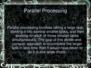
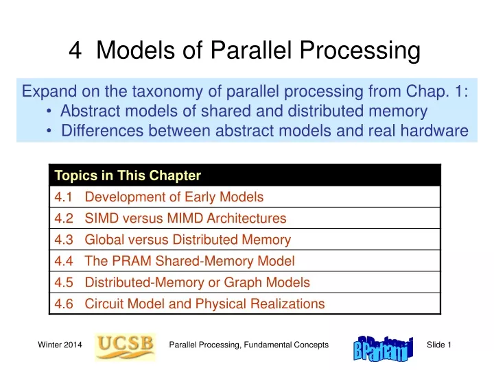
1. 4 Models of Parallel Processing • Expand on the taxonomy of parallel processing from Chap. 1: • Abstract models of shared and distributed memory • Differences between abstract models and real hardware Parallel Processing, Fundamental Concepts

2. 4.1 Development of Early Models • Associative processing (AP) was perhaps the earliest form of parallel processing. • Associative or content-addressable memories (AMs, CAMs), allow memory cells to be accessed based on contents rather than their physical locations within the memory array. • AM/AP architectures are essentially based on incorporating simple processing logic into the memory array so as to remove the need for transferring large volumes of data through the limited-bandwidth interface between the memory and the processor (the von Neumann bottleneck). Parallel Processing, Fundamental Concepts

3. 4.1 Development of Early Models • Early associative memories provided two basic capabilities: • Masked search, or looking for a particular bit pattern in selected fields of all memory words and marking those for which a match is indicated. • Parallel write, or storing a given bit pattern into selected fields of all memory words that have been previously marked. Comparand 100111010110001101000 Mask Memory array with comparison logic Parallel Processing, Fundamental Concepts

4. Fig. 4.2 The Flynn-Johnson Classification Revisited Fig. 4.1 The Flynn-Johnson classification of computer systems. Parallel Processing, Fundamental Concepts

5. The Flynn-Johnson Classification Revisited Parallel Processing, Fundamental Concepts

6. The Flynn-Johnson Classification Revisited Figure 4.2. Multiple Instruction streams operating on a single data stream • Various transformations are performed on each data item before it is passed on to the next processor(s). • Successive data items can go through different transformations • Data-dependent conditional statements Parallel Processing, Fundamental Concepts

7. 4.2 SIMD versus MIMD Architectures Within the SIMD category, two fundamental design choices exist: • Synchronous versus asynchronous: • In a SIMD machine, each processor can execute or ignore the instruction being broadcast based on its local state or data-dependent conditions. • This leads to some inefficiency in executing conditional computations. • For example, an “if-then-else” statement is executed by first enabling the processors for which the condition is satisfied and then flipping the “enable” bit before getting into the “else” part. Parallel Processing, Fundamental Concepts

8. 4.2 SIMD versus MIMD Architectures • A possible cure is to use the asynchronous version of SIMD, known as SPMD (single-program, multiple data), where each processor runs its own copy of the common program. The advantage of SPMD is that in an “if-then-else” computation, each processor will only spend time on the relevant branch. • The disadvantages include the need for occasional synchronization and the higher complexity of each processor, which must now have a program memory and instruction fetch/decode logic. Parallel Processing, Fundamental Concepts

9. 4.2 SIMD versus MIMD Architectures SIMD: Processing the “If statement” Consider the following block of code, to be executed on four processors being run in SIMD mode. These are P0, P1, P2, and P3. if (x > 0) then y = y + 2 ; else y = y – 3; Suppose that the x values are as follows (1, –3, 2, –4). Here is what happens. What one wants to happen is possibly realized by the SPMD architecture. Parallel Processing, Fundamental Concepts

10. 4.2 SIMD versus MIMD Architectures • Custom- versus commodity-chip SIMD: • A SIMD machine can be designed based on commodity (off-the-shelf) components or with custom chips. • In the first approach, components tend to be inexpensive because of mass production. However, such general-purpose components will likely contain elements that may not be needed for a particular design. • Custom components generally offer better performance but lead to much higher cost in development. Parallel Processing, Fundamental Concepts

11. 4.2 SIMD versus MIMD Architectures • Within the MIMD class, three fundamental issues are: • Massively or moderately parallel processor. • Is it more cost-effective to build a parallel processor out of a relatively small number of powerful processors or a massive number of very simple processors. • Referring to Amdahl’s law, the first choice does better on the inherently sequential part of a computation while the second approach might allow a higher speed-up for the parallelizable part. Parallel Processing, Fundamental Concepts

12. 4.2 SIMD versus MIMD Architectures • Tightly versus loosely coupled MIMD: • Which is a better approach to high performance computing, that of using specially designed multiprocessors/ Multi computers or a collection of ordinary workstations that are interconnected by commodity networks ? • Explicit message passing versus virtual shared memory: • Which scheme is better, that of forcing the users to explicitly specify all messages that must be sent between processors or to allow them to program in an abstract higher-level model, with the required messages automatically generated by the system software? Parallel Processing, Fundamental Concepts

13. Options: Crossbar Bus(es) MIN Bottleneck Complex Expensive 4.3 Global versus Distributed Memory Fig. 4.3 A parallel processor with global memory. Parallel Processing, Fundamental Concepts

14. 4.3 Global versus Distributed Memory • Global memory may be visualized as being in a central location where all processors can access it with equal ease. • Processors can access memory through a special processor-to-memory network. • The interconnection network must have very low latency, because access to memory is quite frequent. Parallel Processing, Fundamental Concepts

15. 4.3 Global versus Distributed Memory A global-memory multiprocessor is characterized by the type and number p of processors, the capacity and number m of memory modules, and the network architecture • Crossbar switch • O(pm) complexity, and thus quite costly for highly parallel systems • 2. Single or multiple buses • the latter with complete or partial connectivity 3. Multistage interconnection network Parallel Processing, Fundamental Concepts

16. 4.3 Global versus Distributed Memory • One approach to reducing the amount of data that must pass through the processor-to memory interconnection network is to use a private cache memory of reasonable size within each processor. • locality of data access, repeated access to the same data, and the greater efficiency of block, as opposed to word-at-a-time, data transfers. • The use of multiple caches gives rise to the cache coherence problem. Parallel Processing, Fundamental Concepts

17. 4.3 Global versus Distributed Memory Challenge: Cache coherence Fig. 4.4 A parallel processor with global memory and processor caches. Parallel Processing, Fundamental Concepts

18. 4.3 Global versus Distributed Memory • With single cache, the write through policy can keep the two • data copies consistent. For examples: • Do not cache shared data at all or allow only a single cache copy • Do not cache “writeable” shared data or allow only a single cache copy • Use a cache coherence protocol Parallel Processing, Fundamental Concepts

19. 4.3 Global versus Distributed Memory • A collection of p processors, each with its own private memory, communicates through an interconnection network. • The latency of the interconnection network may be less critical, as each processor is likely to access its own local memory most of the time. • Because access to data stored in remote memory modules involves considerably more latency than access to the processor’s local memory, distributed-memory MIMD machines are sometimes described as non uniform memory access (NUMA) architectures. Parallel Processing, Fundamental Concepts

20. 4.3 Global versus Distributed Memory Some Terminology: NUMA Non uniform memory access (distributed shared memory) UMA Uniform memory access (global shared memory) COMA Cache-only memory arch Fig. 4.5 A parallel processor with distributed memory. Parallel Processing, Fundamental Concepts

21. 4.4 The PRAM Shared-Memory Model • The theoretical model used for conventional or sequential computers (SISD class) is known as the random-access machine (RAM) • The abstraction consists of ignoring the details of the processor-to-memory interconnection network and taking the view that each processor can access any memory location in each machine cycle, independent of what other processors are doing. The problem multiple processors attempting to write into a common memory location must be resolved in some way Parallel Processing, Fundamental Concepts

22. 4.4 The PRAM Shared-Memory Model Fig. 4.6 Conceptual view of a parallel random-access machine (PRAM). Parallel Processing, Fundamental Concepts

23. 4.4 The PRAM Shared-Memory Model • In the SIMD variant, all processors obey the same instruction in each machine cycle; however, because of indexed and indirect (register-based) addressing, they often execute the operation that is broadcast to them on different data. In view of the direct and independent access to every memory location allowed for each processor, the PRAM model depicted highly theoretical • Because memory locations are too numerous to be assigned individual ports on an interconnection network, blocks of memory locations (or modules) would have to share a single network port. Parallel Processing, Fundamental Concepts

24. 4.4 The PRAM Shared-Memory Model PRAM Cycle: All processors read memory locations of their choosing All processors compute one step independently All processors store results into memory locations of their choosing Fig. 4.7 PRAM with some hardware details shown. Parallel Processing, Fundamental Concepts

25. 4.5 Distributed-Memory or Graph Models Given the internal processor and memory structures in each node, a distributed-memory architecture is characterized primarily by the network used to interconnect the nodes Important parameters of an interconnection network include: • Network diameter • Bisection (band)width • Vertex or node degree Parallel Processing, Fundamental Concepts

26. 4.5 Distributed-Memory or Graph Models • Network diameter • The network diameter is more important with store-and-forward routing • 2. Bisection (band)width • This is important when nodes communicate with each other in a random fashion • Vertex or node degree • The node degree has a direct effect on the cost of each node with the effect being more significant for parallel ports containing several wires or when the node is required to communicate over all of its ports at once. Parallel Processing, Fundamental Concepts

27. 4.5 Distributed-Memory or Graph Models Fig. 4.8 The sea of interconnection networks. Parallel Processing, Fundamental Concepts

28. –––––––––––––––––––––––––––––––––––––––––––––––––––––––––––––––––––––––––––––––––––––––––––––––––––––––––––––––––––––––––––––––––– Number Network Bisection Node Local Network name(s) of nodes diameter width degree links? ––––––––––––––––––––––––––––––––––––––––––––––––––––––––––––––––– 1D mesh (linear array) kk – 1 1 2 Yes 1D torus (ring, loop) kk/2 2 2 Yes 2D Mesh k2 2k – 2 k 4 Yes 2D torus (k-ary 2-cube) k2k 2k 4 Yes1 3D mesh k3 3k – 3 k2 6 Yes 3D torus (k-ary 3-cube) k3 3k/2 2k2 6 Yes1 Pyramid (4k2 – 1)/3 2 log2 k 2k 9 No Binary tree 2l – 1 2l – 2 1 3 No 4-ary hypertree 2l(2l+1 – 1) 2l 2l+1 6 No Butterfly 2l(l + 1) 2l 2l 4 No Hypercube 2ll 2l–1l No Cube-connected cycles 2l l2l 2l–1 3 No Shuffle-exchange 2l2l – 1  2l–1/l 4 unidir. No De Bruijn 2ll 2l/l 4 unidir. No –––––––––––––––––––––––––––––––––––––––––––––––––––––––––––––––– 1 With folded layout Some Interconnection Networks (Table 4.2) Parallel Processing, Fundamental Concepts

29. 4.5 Distributed-Memory or Graph Models In LogP model, the communication architecture of parallel computer is captured in four parameters: • Latency : • Latency upper bound when a small message (of a few words) is sent from an arbitrary source node to an arbitrary destination node • Overhead: • The overhead, defined as the length of time when a processor is dedicated to the transmission or reception of a message, thus not being able to do any other computation • gap : • The gap, defined as the minimum time that must elapse between consecutive message transmissions or receptions by a single processor • Processor: • Processor multiplicity (p in our notation) Parallel Processing, Fundamental Concepts

30. 4.5 Distributed-Memory or Graph Models Because a single bus can quickly become a performance bottleneck as the number of processors increase, a of multiple bus architecture are available for reducing bus traffic. Fig. 4.9 Example of a hierarchical interconnection architecture. Parallel Processing, Fundamental Concepts

31. 4.6 Circuit Model and Physical Realizations • The best thing is to model the machine at the circuit level, so that all computational and signal propagation delays can be taken into account. • It is impossible for a complex supercomputer , both because generating and debugging detailed circuit specifications are not much easier than a full-blown implementation and because a circuit simulator would take eons to run the simulation. Parallel Processing, Fundamental Concepts

32. 4.6 Circuit Model and Physical Realizations • A more precise model, particularly if the circuit is to be implemented on a dense VLSI chip, would include the effect of wires, in terms of both the chip area they consume (cost) and the signal propagation delay between and within the interconnected blocks (time) • It is seen that for the hypercube architecture, which has nonlocal links, the inter processor wire delays can dominate the intra processor delays, thus making the communication step time much larger than that of the mesh- and torus-based architectures. Parallel Processing, Fundamental Concepts

33. 4.6 Circuit Model and Physical Realizations Fig. 4.10 Intrachip wire delay as a function of wire length. Parallel Processing, Fundamental Concepts

34. 4.6 Circuit Model and Physical Realizations At times, we can determine bounds on area and wire-length parameters based on network properties, without having to resort to detailed specification and layout with VLSI design tools. For example in 2D VLSI implementation, the bisection width of a network yields a lower bound on its layout area in an asymptotic sense. If the bisection width is B, the smallest dimension of the chip should be at least Bw, where w is the minimum wire width (including the mandatory interwire spacing) Parallel Processing, Fundamental Concepts

35. 4.6 Circuit Model and Physical Realizations • Power consumption of digital circuits is another limiting factor. Power dissipation in modern microprocessors grows almost linearly with the product of die area and clock frequency (both steadily rising) and today stands at a few tens of watts in high-performance designs. • Even if modern low-power design methods succeed in reducing this power by an order of magnitude, disposing of the heat generated by 1 M such processors is indeed a great challenge. Parallel Processing, Fundamental Concepts

36. Pitfalls of Scaling up(Fig. 4.11) If the weight of ant grows by a factor of one trillion, the thickness of its legs must grow by a factor of one million to support the new weight Ant scaled up in length from 5 mm to 50 m Leg thickness must grow from 0.1 mm to 100 m Parallel Processing, Fundamental Concepts