Download

1 / 12
140 likes | 273 Views
BUTTERFLY VALVE LOSSES. STEPHEN “DREW” FORD P6.160 13 FEB 2007. P6.160. GIVEN: The butterfly valve losses in Fig. 6.19b may be viewed as a Bernoulli obstruction device, as in Fig. 6.39.

E N D
BUTTERFLY VALVE LOSSES STEPHEN “DREW” FORD P6.160 13 FEB 2007
P6.160 • GIVEN: The butterfly valve losses in Fig. 6.19b may be viewed as a Bernoulli obstruction device, as in Fig. 6.39. • FIND: First fit the Kmean versus the opening angle in Fig6.19b to an exponential curve. Then use your curve fit to compute the “discharge coefficient” of a butterfly valve as a function of the opening angle. Plot the results and compare them to those for a typical flowmeter.
View of the butterfly valve from downstream Using the as the degree of the opening for the variable in out equation.
Fig 6.19(b) Using these values as the original K’s
ASSUMPTIONS • The velocity through the valve is different than the velocity in the entire pipe due to the small silver opening in the valve. • Steady • Incompressible • Frictionless • Continuous
The problem states using Eq. 104 may be helpful. Where At is the area of the silver in the valve. This area is Found to be (1-cos()) The continuity equation gives us: Q = ApVp = AtVt
Manipulation of the continuity equation in terms of the Velocity in the Valve.
The minor losses in valves can be measured by finding “the ratio of the head-loss through the device to the velocity head of the associated piping system.” , K is the dimensionless loss coefficient
The problem states that using the Velocity through the valve will give a better K value. So multiplying the original K by a value of (Vpipe/Vvalve)2 which is a mathematical “1” gives a new equation for K. Which yields the new equation for K
Finding the curve fit lines of the original K values and plug in it in to the Koptimal equation. These curve fit equations are: K1 = 1101.9e-0.0978 (1-cos())2 K2 = 1658.3e-0.1047 (1-cos())2 K3 = 1273.3e-0.1919 (1-cos())2 The calculated values of the K of three different manufactures from the original K values form Fig. 6.19b.
The graph of all 3 manufacture’s valves with the new K values.
Biomedical Application Patients who suffer from valvular diseases in the heart may require replacing the non-functioning valve with an artificial heart valve. These valves keep the large one-dimensional flow going. Fluid mechanics plays a large role in designing these valve replacements, which require minimal pressure drops, minimize turbulence, reduce stresses, and not create flow separations in the vicinity of the valve.