Download

1 / 68
710 likes | 941 Views
Perfect Competition. Assumptions of Perfect Competition. Homogeneous or identical products – every seller’s product is the same as every other seller’s product. Many small independent firms Easy entry & exit into the industry – all resources are perfectly mobile.

E N D
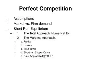
Assumptions of Perfect Competition • Homogeneous or identical products – every seller’s product is the same as every other seller’s product. • Many small independent firms • Easy entry & exit into the industry – all resources are perfectly mobile. • Firms, consumers, & resource owners have perfect knowledge of relevant economic & technical data.
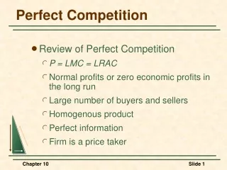
The perfectly competitive firm is a price taker that sells its product at the market price. Why? • If the firm tried to charge more than the market price, it would lose all its business to its competitors who sell the identical product. • The firm can sell as much as it wants at the market price, since it is very small relative to the market. The firm, therefore, has no incentive to charge less than the market price.
Since the perfectly competitive firm always sells its product for the market price, the demand curve for its product is horizontal at the market price. P D Q
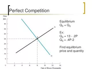
Consider a perfectly competitive firm whose product sells for $10. The firm’s costs are as shown below.
Marginal Revenue is MR =ΔTR/ΔQ . For a perfectly competitive firm, MR is constant & equal to the price of the product.
Notice that when Q = 6, MR=MC and profit is at its maximum.
Notice also that at that profit-maximizing output, price is equal to marginal cost P=MC
P = MC because for the perfectly competitive firm, P = MR & for the profit-maximizing firm, MR = MC.
On a graph, the perfectly competitive firm making a positive economic profit looks like this. The horizontal demand curve lies above the minimum of the ATC curve. MC ATC $ P D = MR Q* Quantity
Sometimes the best the firm can do is break even (make zero economic profits). This occurs when the price (& the demand curve) are at the minimum of the ATC curve. MC ATC $ AVC P D = MR Quantity
What if the demand curve lies below the minimum of the ATC curve but above the minimum of the AVC curve? MC ATC $ AVC P D = MR Quantity
Then the firm will have an economic loss. • However, the firm will still operate. • If the firm were to shut down & produce nothing, its loss would equal its fixed cost. • But since the price is greater than the variable costs per unit (AVC), by operating the firm will be able to cover its variable costs & part of its fixed costs. • So its loss would be smaller than the amount of fixed cost. • So it pays to operate, as long as the price is above the minimum of the average variable cost.
Mathematically, the situation works like this: • P > AVC • So, PQ > AVC (Q), • [Now since AVC = TVC / Q , • AVC (Q) = TVC.] • So, PQ > TVC • TR > TVC • TR – TC > TVC – TC • > TVC – TC • > – TC + TVC • > -1(TC – TVC) • > – TFC If the firm produced nothing, = TR – TC = TR – (TVC+TFC ) = 0 – (0+TFC) = – TFC So the firm does better by operating than by shutting down.
If the price equals the minimum value of the AVC curve, the firm will lose the same amount if it shuts down or if it operates. MC ATC $ AVC P D = MR Quantity
However, if the price is below the minimum of the AVC curve, • the firm is unable to cover even the variable costs, & it should shut down. • It would lose more by operating than by shutting down. • Consequently, the minimum of the AVC curve is called the shutdown point.
Graphically, the firm’s horizontal demand curve lies below the minimum of the AVC curve: MC ATC $ AVC P D = MR Quantity
Positive economic profits • Break even • Operate at a loss • Lose same amount if operate or shutdown • Shutdown So we have these five possible cases: MC ATC $ AVC P1 P2 P3 P4 P5 Quantity
Using this information and the fact that the firm maximizes profits by producing where MR = MC, we can determine the firm’s short run supply curve.
If the price is P1, the firm produces output Q1, where MR = MC.(The numbering of the prices in the upcoming slides does not correspond to the numbering in our 5 case discussion.) ATC MC AVC $ D1 = MR1 P1 Quantity Q1
If the price is P2, the firm produces output Q2 . ATC MC $ AVC D2= MR2 P2 Quantity Q2
If the price is P3, the firm produces output Q3. MC ATC $ AVC P3 D3 = MR3 Quantity Q3
If the price is P4, the firm produces output Q4. MC ATC $ AVC P4 D4 = MR4 Quantity Q4
If the price is P5, the firm produces output Q5 (or shuts down – it loses the same amount either way). MC ATC $ AVC P5 D5 = MR5 Quantity Q5
So in determining the quantity the firm would supply at each price, we have actually traced out the points of the MC curve above the minimum of the AVC curve. MC ATC $ AVC Quantity
So this is the firm’s short run supply curve. S Price Quantity
S2 S3 S4 S5 S1 To determine the industry or market short run supply curve, horizontal sum the individual firms’ supply curves. Price Industry supply curve Quantity
S2 S3 S4 S5 S1 That means that for each price, we add the amounts all the firms are willing to supply. For example, if there are five firms who at a price of $25 will supply 10, 20, 30, 40, & 50 units each, the total supplied by the industry at that price is 10 + 20 + 30 + 40 + 50 = 150 . Price Industry supply curve 25 10 20 30 40 50150 Quantity
How do perfectly competitive firms & industries adjust to changes in demand conditions & what are the implications for the long run market supply curve? Let’s start with the simplest case, which is the constant cost industry.
Constant Cost Industry an industry in which costs of production remain constant as industry output expands
Start with the market. Market P S P0 D Q* Q
MC P ATC D= MR P0 q* q Put in a typical firm in long run equilibrium (zero profits). Market Firm P S P0 D Q* Q
Suppose demand increases. Firm Market MC P ATC S D= MR P0 P0 D’ D Q* Q q* q
Price rises and profits are made. Firm Market MC P ATC S P1 D1= MR1 P1 D= MR P0 P0 D’ D Q* Q1 Q q* q1 q
New firms enter the industry, increasing supply. Firm Market MC P ATC S S’ P1 D1= MR1 P1 D= MR P0 P0 D’ D Q*Q1 Q q* q1 q
Price falls to original level, & profits return to zero. Firm Market MC P ATC S S’ P1 D1= MR1 P1 D= MR P0 P0 D’ D Q* Q1 Q2 Q q* q
The Long Run Supply Curve • The initial market point and the final one are long run equilibrium points and therefore are on the long run supply curve for this industry. • (The middle point - the black one - is not on the long run supply curve, since it is not a long run equilibrium point.) • For a constant cost industry, the long run supply curve is a horizontal line.
The Long Run Supply Curve Market P S S’ P1 long run supply curve P0 D’ D Q* Q1 Q2 Q
Increasing Cost Industry an industry in which costs of production increase as industry output expands
Start with the market. Market P S P0 D Q* Q
Put in a typical firm in long run equilibrium (zero profits). Firm Market MC P P ATC S D= MR P0 P0 D Q* Q q* q
Suppose demand increases. Market Firm MC P ATC S D= MR P0 P0 D’ D Q* Q q* q
Price rises and profits are made. Firm Market MC P ATC S P1 D1= MR1 P1 D= MR P0 P0 D’ D Q* Q1 Q q* q1 q
New firms enter the industry, increasing supply. Firm Market MC P ATC S S’ P1 D1= MR1 P1 D= MR P0 P0 D’ D Q*Q1 Q q* q1 q
However, as industry output expands, demand for the inputs rises. The prices of the inputs increase, and therefore production costs increase. • So we see an upward shift in the cost curves.
Cost curves shift upward. Firm Market MC1 ATC1 P ATC S S’ P1 D1= MR1 P1 D= MR P0 P0 MC D’ D Q*Q1 Q q* q1 q