Download

1 / 54
540 likes | 561 Views
Learn methods to assess the strength of relationships between nominal or ordinal variables, using chi-square test and association measures like lambda and gamma.

E N D
Chapter 16 Aids for the Interpretation of Contingency Tables
Chapter 15 instructed us on the general method for constructing and analyzing contingency tables or cross-tabulations, focusing on procedures for percentaging and determining whether two variables measured at the nominal or ordinal level are associated statistically. • Chapter 16 will provide us with details on the methods for assessing the strength of a relationship between a pair of nominal or ordinal variables in a contingency table. • These techniques are not substitutes but supplements to those presented in Chapter 15. • Methods here are used to further understand the relationship between two variables measured at the nominal or ordinal level. Introduction
The chapter is divided into three major segments. • The 1st part is devoted to the chi-square test. • The chi-square test: • Is a test of statistical significance for relationships between variables measured at the nominal or ordinal level. • Assesses whether the relationship observed in a cross-tabulation in a sample of data is sufficiently strong to infer that a relationship is likely to exist in the full population. Introduction
The chapter is divided into three major segments. • The 2nd part of the chapter expands to methods for evaluating the strength of the relationship between two variables. • The most straightforward of these techniques is the percentage difference, which was introduced in Chapter 15 • The 3rd and final portion of the chapter explains measures of association: • Individual statistics that summarize the strength of a relationship demonstrated in a cross-tabulation. • The chapter presents a detailed development of frequently used measures of association: lambda and Cramér’s V for nominal-level variables; and gamma, Kendall’s tau-b and tau-c, and Somers’s dyx and dxy for ordinal-level variables. Introduction
Statistical significance is a procedure for establishing the degree of confidence that one can have in making an inference from a sample to its parent population. • You’ve learned that there is a correspondence between results obtained in a sample of data and the actual situation in the population that the sample is intended to represent • The chi-square test is a procedure used to evaluate the level of statistical significance achieved by a bivariate relationship in a cross-tabulation. • The chi-square test procedure assumes that there is no relationship between the two variables in the population and determines whether any apparent relationship obtained in a sample cross-tabulation is attributable to chance. The Chi-Square Test: Statistical Significance for Contingency Tables
This procedure involves three steps: • First,expected frequencies are calculated for each cell in the contingency table predicated on the assumption that the two variables are unrelated in the population. • Second, based on the difference between the expected frequency and the actual frequency observed in each table cell, a test statistic called the chi-square is computed. • The expected frequencies assume there is no relationship between the two variables, so the greater the deviation between them (expected frequencies) and the actual frequencies, the greater is the departure of the observed relationship from the null hypothesis • The greater is our confidence in inferring the existence of a relationship between the two variables in the population. • Third, the chi-square value computed for the actual data is compared with a table of theoretical chi-square values calculated and tabulated by statisticians. • This comparison allows the analyst to determine the precise degree of confidence that he or she can have in inferring from the sample cross-tabulation that a relationship exists in the parent population. The Chi-Square Test: Statistical Significance for Contingency Tables
Example: Incompetence in the Federal Government? • A disgruntled official working in the personnel department of a large federal bureaucracy is disturbed by the level of incompetence she perceives in the leadership of the organization. She is convinced that incompetence rises to the top, and she shares this belief with a coworker over lunch. The latter challenges her to substantiate her claim. To prove her claim she: • Selects a random sample of 400 people employed by the organization (personnel files). • Based on formal education and civil service examination scores she classifies them into three levels of competence (low, medium, or high) • Based on their General Schedule (GS) ratings and formal job descriptions, she classifies them into three categories of hierarchical position in the organization (low, medium, or high). • The cross-tabulation of these two variables are in the adjacent table (16.1). The official would like to know whether she legitimately can infer from this sample cross-tabulation that a relationship exists competence and hierarchical between position in the population of all workers in the organization. Cross-Tabulation of Competence & Hierarchy
She decides to perform the chi-square test following these procedural steps: • Step 1: Compute expected frequencies for each cell of the cross- tabulation based on the null hypothesis: “competence and hierarchical position are not related in the population”. • Note: If the table has been percentaged, then the data must be converted to raw frequencies before calculation of the expected frequencies. Expected frequencies must be calculated on the basis of the raw figures. • If the two variables were unrelated the distribution of hierarchical position would be the same in each category of competence as in the sample as a whole. • In other words, in each level of competence the percentages of hierarchical position would be identical. • Meaning that: • Competence has no impact on hierarchy • There is a percentage differences of 0% for each category of the dependent variable • The two variables are totally unrelated. Example: Incompetence in the Federal Government?
Example: Incompetence in the Federal Government? Table 16.2 Hypothetical No-Relationship Cross-Tabulation for Chi-Square • Consider the distribution of hierarchical position. Of the 400 people in the sample: • 200 (50%) rank low in position; • 160 (40%) hold medium-level positions; • 40 (10%) are at the top. • Assuming that the null hypothesis is true (no relationship between competence and hierarchy), we would expect to find this same distribution of hierarchical position in each of the categories of competence. • For example if the null hypothesis were true with 152 employees you would expect to find the following in the hierarchy : • Low-level positions, expect 50% or 76.0 (0.50 x 152 = 76.0); • Medium-level positions expect 40% or 60.8 (0.40 x 152 = 60.8); • High-level positions expect 10%, or 15.2 (0.10 x 152 = 15.2). • These are the expected frequencies for the low-competence category.
Step 2: Compute the value of chi-square for the cross-tabulation. The chi-square statistic compares the frequencies actually observed with the expected frequencies throughout the contingency table (presuming no relationship between the variables) • The value of chi-square is found by: • Taking the difference between the observed and expected frequencies for each table cell, • Squaring this difference • Dividing the squared difference by the expected frequency • Summing these quotients across all cells of the table. • For example, in the low competence–low hierarchy cell of Table 16.1, the observed frequency is 113, as compared with an expected frequency of 76.0. • Thus (113 - 76.0)2 ÷ 76.0 = 18.01, as shown in the next slide in the last column of the table (16.3). Example: Incompetence in the Federal Government?
Example: Incompetence in the Federal Government? • Table 16.3 Calculations for Expected Frequencies & Chi-Square – calculation’s virtue is that they yield the value of chi-square, whose theoretical distribution is well known and can be used to evaluate the statistical significance of the relationship found in the contingency table. This table indicates that the value of chi-square for the competence– hierarchy cross- tabulation is 89.20.
Step 3: Compare the value of chi-square computed for the actual cross-tabulation with the appropriate value of chi-square tabulated in the table of theoretical values. The table of chi-square values is presented in Table 4 in the Statistical Tables at the back of this book. • To find the appropriate theoretical value of chi-square in this table for an actual contingency table, two pieces of information must be specified: • The degrees of freedom associated with the table • The level of statistical significance desired. • The degrees of freedom is simply a number that gives some idea of the size of the empirical contingency table under study. • Found by multiplying one less than the number of rows in the table by one less than the number of columns (ignoring both marginal rows and columns). • Current example, the number of rows (3) and the number of columns (3), so (3–1) x (3 -1) = 2 x 2 = 4 degrees of freedom. • In the Statistical Tables, Table 4, the degrees of freedom (df) are printed down the far left column of the table. Example: Incompetence in the Federal Government?
Once the proper theoretical value of chi-square is determined a critical decision can be made: • “Whether the existence of a relationship can be inferred in the population of all agency employees” • Based on the sample cross-tabulation between competence and hierarchical position • The table of theoretical values (Statistical Tables, Table 4) consists of minimum values of chi-square that must be obtained in empirical contingency tables in order to infer, with a given level of confidence (statistical significance), that a relationship exists in the population. Example: Incompetence in the Federal Government?
You should commit the following decision rules for chi-square to memory, if the value of: • Chi-square exceeds the appropriate minimum value in the chi-square distribution table, taking into account the degrees of freedom; reject the null hypothesis. • Chi-square does not exceed the appropriate minimum value in the chi-square distribution table, taking into account the degrees of freedom; cannot reject the null hypothesis. • Here the value of chi-square is 89.20, which is far greater than the appropriate minimum value stipulated by Table 4 with 4 degrees of freedom (9.49), allowing a 5% chance of error, so we can infer that a relationship does exist between competence and hierarchical position in the population. • If chi-square failed to surpass the minimum, the null hypothesis of no relationship in the population could not have been rejected (no relationship b/t competence and hierarchy) Example: Incompetence in the Federal Government?
The level of statistical significance is determined by the public or non-profit manager according to his or her assessment of the decision-making situation • Exact probability of error that the administrator is willing to tolerate in making an inference from the sample cross-tabulation to the parent population in the long run • If the researcher selects the frequently used level of .05, then there is a probability of 5% that in the long run, an inference will be made that a relationship exists in the population when in fact it does not. • If the manager were to make 20 decisions based on the 5% rule, one is likely to be in error, and the other 19 are likely to be correct. Although the manager cannot be certain about any particular decision, she or he can be 95% confident in the long run. • In the Statistical Tables, Table 4, the level of statistical significance (abbreviated P, for probability) is printed along the top of the table; these values cut off the specified area of the curve. • In the table, you’ll find the theoretical value of chi-square for 4 df, allowing a probability of error of 5% (i.e., a level of statistical significance of .05) is equal to 9.49. Example: Incompetence in the Federal Government?
Example: Incompetence in the Federal Government? • The chi-square test is very useful, but the preceding example illustrates one of its primary limitations. • The test led to the conclusion that a relationship does exist between competence and hierarchical position in the population of agency employees. ‘ • But the researcher hypothesized that this relationship is inverse (negative): the less the competence of the employee, the higher the level of the position attained in the hierarchy of the organization. • When the cross-tabulation of these two variables in the sample of employees has been percentaged correctly the relationship between competence and hierarchical position is found to be positive (as competence increases, position in the hierarchy also increases). • Meaning the existence of a relationship can be inferred in the population (the opposite direction of the one hypothesized by the researcher) • The disgruntled official’s hypothesis is incorrect. Table 16.2 Hypothetical No-Relationship Cross-Tabulation for Chi-Square
The important point illustrated by this example is not that the chi-square test yields erroneous information, but that it yields information which is limited. • The test is based solely on the deviation of an observed cross-tabulation from the condition of no relationship or statistical independence. • The chi-square test is totally insensitive to the nature and direction of the relationship actually found in the contingency table. • Managers must be careful not to jump to the conclusion that a significant value of chi-square calculated in a table indicates that the two variables are related in the hypothesized manner in the population. It may or it may not. • Supplementary analytical procedures, such as percentaging the contingency table and computing a measure of association (later in this chapter), are necessary to answer this question. • Remember, the techniques presented in this chapter are supplements, not substitutes. Limitations of the Chi-Square Test
The other limitations of the chi-square test are typical of tests of statistical significance in general (see Part IV, “Inferential Statistics”). • First, the chi-square test requires a method of sampling from the population—simplerandom sampling—that sometimes cannot be satisfied. • Second, the value of chi-square calculated in a cross-tabulation is markedly inflated by sample size. • In large samples, relationships are sometimes found to be statistically significant even when they are weak in magnitude. Hence, the test is not very discriminating. • Third, the chi-square test is frequently misinterpreted as a measure of strength of relationship, it does not assess the magnitude or substantive importance of empirical relationships. • Instead, it provides information pertaining only to the probability of the existence of a relationship in the population. To be sure, this is valuable information, but it ignores the issue of size of relationship. • It is strongly encouraged that you to use the chi-square test in conjunction with other statistical procedures, especially those designed to evaluate strength of relationship. Limitations of the Chi-Square Test
Two transportation planners are locked in debate regarding the steps that should be implemented to increase ridership on public transportation, particularly line buses. • The first insists that the major reason why people do not ride the bus to work is that they have not heard about it. • She argues in favor of advertisement. • The second believes that the primary obstacle to the success of public transportation is that it is not readily accessible to great masses of potential riders. People will not leave their cars for a system they are unable to reach conveniently. • He argues to expand existing bus routes and design & implement new ones . • Due to the difference in public policy implications and cost the federal government has decided to fund a study to evaluate the relative validity of the two claims. Data were collected from a random sample of 500 individuals. Among other questions, these individuals were asked whether they: • Rode the bus regularly to work • Had learned of the existence of public transportation through advertising, • Lived in close proximity to a bus stop (defined as within three blocks). The Percentage Difference
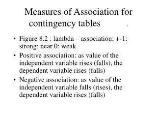
The Percentage Difference • The adjacent table (16.5) presents the cross-tabulations between riding the bus to work and each of the other two variables • The table provides support for the hypotheses of both planners. • Advertising is related positively to ridership. • 33% of those who heard public transportation advertising rode the bus regularly to work • 25% of those who had not heard such advertising rode. • Thus, advertising was associated with an 8% increase in ridership. • Accessibility is related positively to ridership; • 40% of those living in close proximity to a bus stop rode the bus regularly, • 23% of those for whom the bus was less convenient. • Thus, accessibility was associated with a 17% increase in ridership.
Which proposal is likely to have the greater impact on increasing ridership of public transportation? • Accessibility (difference of 17%) seems to have made a larger impact on ridership than advertising (difference of 8%) • Changes in accessibility apparently lead to a larger change in ridership than do changes in advertising. • Stated another way, accessibility is related more strongly to ridership than is advertising. • In general, the greater the percentage difference, the stronger is the relationship between two variables. • So, if the federal government intends to adopt one or the other of the two proposals (but not both) as a measure to increase the ridership of public transportation, these data suggest that improving accessibility is to be preferred. The Percentage Difference
Perfect & Null Relationships • In a cross-tabulation, as the independent variable changes categories, the percentage difference for a given category of the dependent variable may range from 0% to 100%. • % differences of 100 for each of the categories of the dependent variable indicate that the two variables are associated perfectly. • Known independent variable score allows the prediction of dependent variable scores with certainty. • Relationship b/t two variables is perfect if all cases are located in the diagonal cells of contingency table. Two types of prefect relationship exist. If the categories of both variables fall into the diagonal cells: • Sloping downward from the top-left cell to the bottom-right one (ascending order relationship/perfect in the positive direction) • Sloping downward from the top-right cell to the bottom-left one, (relationship is perfect in the negative direction)
Perfect and Null Relationships • In the previous slide: The closer the observed cross-tabulation comes to either of the configurations, the stronger is the association between the two variables. Because changes in the independent variable are hypothesized to be accompanied by changes in the dependent variable, this pattern is called the covariation model of relationship. • At the other extreme (cross-tabulation) percentage differences of 0% within each of the categories of the dependent variable indicate that the independent and dependent variables are not associated. • The more similar the distribution of the dependent variable across each of the categories of the independent variable, the less strongly the two variables are related. • Remember the chi-square test, the strength of relationship between two variables reaches its lowest point when those distributions are identical. • Table 16.2, developed in conjunction with the chi-square test provides an example. The value of the independent variable (competence) does not help in predicting values of the dependent variable (hierarchy) because the percentages are the same for each category of the independent variable. Even if you knew a person’s level of competence, it would not help in predicting her or his position in the hierarchy. Table 16.2 Hypothetical No-Relationship Cross-Tabulation for Chi-Square
Table 16.7 illustrates that in contrast to the single model of perfect association, there are many empirical models of no association.
The discussion of extreme values of association raises a problem with respect to the percentage difference as a measure of strength of relationship. • The strength of the relationship is based only on the endpoint categories of the dependent variable, so the percentage difference does not satisfy this desideratum; • It takes into account only a portion of the data in the table (see Chapter 15). • As a result, in larger cross-tabulations, the choice of the dependent variable category not only is somewhat arbitrary but also can lead to different results representing the strength of relationship between two variables in the same table. • Depending on one’s point of view, the category selected may understate or overstate the actual degree of relationship in the cross-tabulation. • It is recommended (in Chapter 15) that you calculate and report both percentage differences. Perfect and Null Relationships
All statistics have imperfections. However, in spite of its flaws, the percentage difference is possibly the most widely used and easily understood measure of strength of relationship. • Used in combination with the other measures (elaborated in this chapter), percentage difference can be very helpful in evaluating the nature and strength of relationship between two variables (nominal or ordinal level). • An unavoidable consequence of describing,. summarizing or gleaning a distribution into a single representative number or statistic is that some features of the data are captured very well, while others are slighted or overlooked completely. • For this reason, measures presented for understanding bivariate relationships should be treated as complementary rather than exclusive. • In actual data analysis, use those measures that best elucidate the relationship under study. Perfect and Null Relationships
Measures of association are statistics whose magnitude and sign (positive or negative) provide an indication of the extent and direction of relationship between two variables in a cross-tabulation. • In contrast to the percentage difference, measures of association are calculated on the basis of—and take into account—all data in the contingency table. • Measures of association is designed to indicate where an actual relationship falls on the scale from perfect to null. Measures of Association
To facilitate interpretation, statisticians define measures of association so that they follow these four conventions: • If the relationship between the two variables is perfect, the measure equals +1.0 (positive relationship) or -1.0 (negative relationship). • If there is no relationship between the two variables, the measure equals .0. • The sign of the measure indicates the direction of the relationship. • A value greater than zero (a positive number) corresponds to a positive relationship; a value less than zero (a negative number) corresponds to a negative relationship. • The stronger the relationship between the two variables, the greater is the magnitude of the measure. The absolute value of the statistic (ignoring sign) is what matters in assessing magnitude. A relationship measuring -.75 (or .75) is larger than one measuring -.25 (or .25). Measures of Association
The concept of direction (or sign) of relationship assumes that the categories of the variables are ordered (they increase or decrease in substantive meaning), • For this reason this concept can be applied only to relationships between variables measured at the ordinal or interval levels. • Direction of relationship has no meaning for nominal variables because the categories (for example, religion) have no numerical ordering. • Based on the properties of measurement for each type of variable (interval, ordinal, and nominal) different measures of association have been developed. • Some interval measures are considered in Part VI on regression analysis. • The remainder of this chapter describes several ordinal and nominal measures of association. Measures of Association
An Ordinal Measure of Association: Gamma • Note: It is cumbersome to compute any of the ordinal measures of association by hand, even with the aid of a (nonprogrammable) calculator. the best strategy is to use a computer (statistical package programs) or a programmable calculator. • Computation of gamma is one of the more easily calculated ordinal measures of association. • Also, several other of the most frequently used measures of ordinal association (the tau statistic of Kendall and the d statistics of Somers) are illustrated. • Gamma will be used to assess the strength of relationship between education and seniority in a small sample of 50 employees in a nonprofit organization. • To calculate the gamma statistic, we must first introduce the idea of paired observations. Consider the two data cases in the table below: • 1). Of an individual in the low education–low seniority cell, and the other • 2). Of an individual in the high education–high seniority cell. • For this pair of cases, as education increases, seniority increases (provides support for the existence of a positive relationship).
An Ordinal Measure of Association: Gamma • If all cases were in these two cells of the table, we would have a perfect positive relationship (see Table 16.6). This situation is called a concordant pair of cases. • Now consider two different data cases in Table 16.8: • One of an individual in the low education–high seniority cell • The other of an individual in the high education–low seniority cell. • If the pair of cases is ranked inconsistently on education and seniority (education increases, seniority decreases, and vice versa), there is support for the existence of a negative relationship between the two variables. This situation is called a discordant pair of cases. • If all cases fell into these two table cells, we would have a perfect negative relationship.
To obtain gamma take the difference between the number of concordant (consistently ordered pairs) and the number of discordant (inconsistently ordered pairs) in the cross-tabulation. • If the number of concordant pairs exceeds the number of discordant pairs there is greater support for a positive relationship in the table (difference is positive/gamma statistic will have (+) sign. • If the number of concordant pairs is less than the number of discordant pairs, there is greater support for a negative relationship (difference is negative/ gamma statistic will have (-) sign • The larger the difference between the number of concordant and the number of discordant pairs, the greater is the association between the two variables, and the greater is the magnitude (absolute value) of gamma. Direction of the relationship is not important. An Ordinal Measure of Association: Gamma
To calculate gamma there are three steps: • Step 1: Calculate the number of concordant pairs and the number of discordant pairs of cases in the cross-tabulation. In a small cross-tabulation the calculation is not difficult (i.e., Table 16.8). Consider the concordant pairs: • First, low education–low seniority cell of the table (20 cases) and; • Second concordant pairs: high education–high seniority cell (15 cases) • Because each pairing of cases from these two table cells yields a concordant pair, in all there are 20 x 15 = 300 concordant pairs in Table 16.8. • Now consider the discordant pairs. There are 10 cases in the • First, high education–low seniority cell of the table (10 cases) and; • Second discordant pairs: low education–high seniority cell (5 cases). • Because each pairing of cases from these two table cells gives a discordant pair, there are 10 x 5 = 50 discordant pairs in Table 16.8. An Ordinal Measure of Association: Gamma
To calculate gamma there are three steps: • Step 2: Calculate the difference between the number of concordant pairs and the number of discordant pairs. • It is evident that the relationship between education and seniority in Table 16.8 is positive because there are more concordant than discordant pairs. The difference between them is 300 - 50 = 250. • This simple difference is not very meaningful for interpreting the relative strength of relationship. • It’s misleading to compare the difference obtained from a small contingency table with that of a larger table or a tables with many more cases. The latter will generate so many more pairs of case. An Ordinal Measure of Association: Gamma
An Ordinal Measure of Association: Gamma • Step 3: Standardizing the Measure • Divide the difference between the number of concordant pairs and the number of discordant pairs by their sum. Division by the sum of the number of concordant pairs and the number of discordant pairs in the cross-tabulation ensures that gamma will vary between -1.0 and +1.0 (it will also follow the other conventions for measures of association discussed earlier). The three steps for calculating gamma can be summarized in a formula: • Gamma= (# of concordant pairs - # of discordant pairs) ÷ (# of concordant pairs + # of discordant pairs) • (300 – 50) ÷ (300 + 50) = 250 ÷ 350 = 0.71 • Gamma indicates a relatively strong positive relationship between education and seniority in the sample of employees of the Southeast Animal Rights Association. • Once the original cross-tabulation has been percentaged, there is further support found for this conclusion. The percentaged table below shows that as education increased, employees were more likely to have high seniority by a difference of 60% – 20% = 40%.
Several other commonly used measures of association for ordinal-level variables have a derivation and interpretation similar to gamma’s. These include: • Kendall’s tau-b and tau-c • Somers’s dyx and dxy. • These measures are easy for the computer to calculate (statistical package programs), but they are very cumbersome to calculate by hand, for this reason there will only be an explanation their use and an interpretation. Other Ordinal Measures of Association: Kendall’s tau-b and tau-c and Somers’s dyx and dxy
Like gamma, all of these measures are based on comparing the number of concordant pairs with the number of discordant pairs in the contingency table. Yet they differ from gamma because they take into account pairs of observations in the table that are tied on one or both of the variables. • For example, a case in the low education–low seniority cell of the table is tied with a case in the low education–high seniority cell with respect to education because both cases have the same rank on education. Similarly, a case in the low education–high seniority cell is tied with a case in the high education–high seniority cell with respect to seniority because they both have the same rank on seniority. • Gamma takes into account only concordant and discordant pairs; it ignores tied pairs completely. • The other measures of association are based on a more stringent conception of the types of data patterns in a contingency table that constitute a perfect relationship. • In particular, they will yield lower values for a contingency table to the extent that the table contains pairs of cases tied on the variables. For this reason, unless a contingency table has no tied pairs (a very rare occurrence), gamma will always be greater than tau-b, tau-c, dyx, and dxy. Other Ordinal Measures of Association: Kendall’s tau-b and tau-c and Somers’s dyx and dxy
Kendall’s tau-bis an appropriate measure of strict linear relationship for “square tables” (same number of rows as columns). The calculation of tau-b takes into account pairs of cases tied on each of the variables in the contingency table. • For the education–seniority cross-tabulation in Table 16.8, the calculated value of tau-b is .41. • Kendall’s tau-c is an appropriate measure of linear relationship for “rectangular tables” (different numbers of rows and columns). Note that in such a cross-tabulation, no clear diagonal exists for either a perfect positive or a perfect negative relationship (see Table 16.6)—so a different measure of association is needed for this situation. • In the current example, tau-c is .40 (tau-b is preferred because the table is square). • Somers’s dyx presumes that seniority is the dependent variable and yields lower values to the degree that cases are tied on this variable only. The logic is that a tie on seniority indicates that a change in the independent variable (education) does not lead to a change in seniority as a perfect relationship would predict. • Here, Somers’s dyx is .40. • Conversely, Somers’s dyx presumes that education is the dependent variable and yields lower values to the degree that cases are tied on education only. The reasoning is that a tie on the dependent variable (now education) indicates that a change in the independent variable (now seniority) does not lead to a change in education, as a perfect relationship would predict. In this example, • Somers’s dxy is .42, but it would not be the statistic of choice because the hypothesis was that education (independent variable) leads to seniority (dependent variable), not the reverse. Other Ordinal Measures of Association: Kendall’s tau-b and tau-c and Somers’s dyx and dxy
Recall that the gamma calculated for Table 16.8 is .71, which is much greater than the calculated value of any of the other measures of association. The reason is the tied pairs of cases. In measures of association, gamma will typically yield the largest value, whereas the others will be more modest. Which measure(s) should you use and interpret? In general, the tau measures are used more commonly than are the Somers’s d measures. Many managers prefer to use both gamma and either tau-b or tau-c, depending on whether the contingency table is square or rectangular, respectively. By doing so, the measures give a good idea of the magnitude of the relationship found in the table evaluated according to less stringent and more stringent standards of association. Other Ordinal Measures of Association: Kendall’s tau-b and tau-c and Somers’s dyx and dxy
Ordinal measures of association are based on a covariation model of relationship (extent that two variables change together or covary) • Gamma assess the extent to which increases in one variable are accompanied by increases (positive relationship) or decreases (negative relationship) in a second variable. • Nominal variables do not consist of ordered categories (no sense of magnitude or intensity), application of the covariation model of association to relationships between nominal variables is precluded and a different model of association is required. • A model of association for nominal variables, called the predictability model (model of predictive association). Is based on the ability to predict the category of the dependent variable based on knowledge of the category of the independent variable. • A frequently used nominal measures of association based on the predictability model is Lambda ( it evaluates the extent to which prediction of the dependent variable is improved when the value of the independent variable is known) • The worst case scenario: the independent variable provides no (zero) improvement in predicting the dependent variable • Lambda cannot be negative but ranges from 0.0 to +1.0. Consistent with the idea that relationships between nominal variables do not have direction, only predictability. Measures of association that incorporate the “proportional reduction in error” interpretation are sometimes abbreviated PRE statistics. A Nominal Measure of Association: Lambda
A Nominal Measure of Association: Lambda • Example to illustrate the calculation and interpretation of lambda. Consider the relationship between race (white; nonwhite) and whether an individual made a contribution to the Bureau of Obfuscation’s United Way annual fund drive. • Step 1: Calculate the number of errors in predicting the value of the dependent variable if the value of the independent variable were not known. • First disregard totally the race of the employee (independent variable). If race is disregarded, how many errors will we make in predicting whether the employee made a contribution to the United Way (dependent variable)? • Because more employees made a contribution than did not, our best prediction is “contributed” This prediction is correct for 275 of the 500 employees in the sample who contributed, but it is in error for the remaining 225 who did not contribute. • When the value of the independent variable is not taken into account (disregarded), the proportion of errors made in predicting the dependent variable is 225 ÷ 500 = .45.
A Nominal Measure of Association: Lambda • Step 2: Calculate the number of errors in predicting the value of the dependent variable, this time taking into account the value of the independent variable. • If the race of the employee is now introduced, how much better can we predict contributions to the United Way? • If we knew that an employee was nonwhite, our best prediction would be that he or she made a contribution. We would be correct for 200 of the 300 nonwhites in the sample who made a contribution • We would make errors in predicting for the other 100 who did not. • If an employee is white, we would predict that he or she did not make a contribution. We would be correct for 125 of the 200 whites who did not contribute, leaving 75 errors in prediction for those who did. • Knowing the race of the employee, we would make a total of 100 + 75 = 175 errors in predicting contributions to the United Way in a sample of 500 employees. This procedure yields a proportion of error equal to 175 ÷500 = .35.
A Nominal Measure of Association: Lambda • Step 3: Calculate the rate of improvement in predicting the value of the dependent variable when the value of the independent variable is known • (Step 2) over the original prediction in which the value of the independent variable was ignored (Step 1). • By how much has the rate of error in predicting the dependent variable been reduced by introducing knowledge of the independent variable? • We began with a proportion of error in predicting the dependent variable of 0.45 (not taking into account the independent variable). • By introducing the independent variable, we were able to reduce the proportion of error to 0.35. • How much of an improvement do we have? Compared with the original proportion, this is a rate of improvement in predicting the dependent variable—or proportional reduction in error—of • 0.45 - 0.35÷0.45 = 0.22 which is the value of lambda for Table 16.10. This value suggests a moderate predictive relationship between race and contributions to the United Way.
A Nominal Measure of Association: Lambda • An alternative way to compute lambda is to consider that without knowing the value of the independent variable, we made 225 errors in predicting the dependent variable; and that knowing the independent variable, we made 175 errors, a reduction of 50 errors. Errors in prediction were reduced by the proportion 50 ÷ 225 = .22 (the value of lambda for Table 16.10) • Based on this logic, the formula for lambda can be written • Lamba={(# of errors in prediction of not knowing value of independent variable) - (# of errors in prediction knowing value of independent variable)} ÷ # of errors in prediction not knowing value of independent variable
The chi-square test of statistical significance elaborated at the outset of this chapter is a measure of the existence of a relationship, not its strength. A variety of measures of association for nominal-level variables have been developed based on the chi-square. • The measures include Pearson’s contingency coefficient C, phi-square, Tschuprow’s T, and Cramér’s V. These measures are all related, and many computer statistical packages have been programmed to calculate and show them routinely. • Probably the most useful (and most often used) of the measures is Cramér’s V. It is given by the formula • V = √(chi-square÷mN) • where chi-square = value of chi-square calculated for the contingency table; m = (number of rows in the table - 1) or (number of columns in the table - 1), whichever is smaller; and N = size of the sample. A Nominal Measure of Association Based on Chi-Square: Cramér’s V
Although the formula may seem complicated, it is easy to calculate Cramér’s V, and we do so now for the cross-tabulation in Table 16.1. • V = √(chi-square÷mN) • Step 1: Calculate the value of chi-square for the cross-tabulation. For the data in Table 16.1, the value of chi-square is 89.20 • Step 2: Calculate m. • Determine which is smaller, the number of rows or the number of columns in the cross-tabulation, and subtract 1 from this number. Because Table 16.1 has the same number of rows as columns (3), this choice does not matter in this example. • Subtracting 1 from 3 yields a difference of 2, which is the value of m. A Nominal Measure of Association Based on Chi-Square: Cramér’s V
Step 3: • The remainder of the formula indicates that we must multiply m times N; Divide chi-square (from Step 1) by this product; and take the square root of the result. • m = 2 and N = 400, so m x N = 2 x 400 = 800. • Dividing chi-square (89.20) by this product = 89.20 ÷ 800 = 0.1115; taking the square root of 0.1115 = 0.33, which is the value of Cramér’s V for Table 16.1. • Like all measures of association for nominal-level variables, Cramér’s V is always a positive number (remember that the direction of relationship has no meaning for nominal data). The measure ranges from 0.0, indicating no relationship between the variables, to 1.0, indicating a perfect relationship. A Nominal Measure of Association Based on Chi-Square: Cramér’s V
For the analysis of relationships between variables measured at the ordinal level, researchers generally use ordinal measures of association. • However, if the manager anticipates that the relationship is one not of covariation but of predictability, a nominal measure of association such as lambda can be employed. • This principle follows the Hierarchy of Measurement introduced in Chapter 5. • Example: one might hypothesize that, because jobs at the bottom of the organizational hierarchy tend to be low paying and those at the top tend to be quite stressful, middle-level officials may have the highest level of job satisfaction. • An empirical example is presented in Table 16.11; the data are for staff members of the Inward Institute, a small liberal arts college in central Iowa. Use of Nominal Measures of Association with Ordinal Data
Use of Nominal Measures of Association with Ordinal Data • Because the cross-tabulation in Table 16.11 does not demonstrate a consistent pattern of increase in job satisfaction (dependent variable) with an increase in hierarchy (independent variable), the value of an ordinal measure of association predicated on the covariation logic will be small. • In contrast, because job satisfaction is highly predictable based on the categories of hierarchy, the value of lambda will be large. • If one knows an employee’s level in the hierarchy, then a very good prediction can be made regarding job satisfaction. For example, for those low in hierarchy, predict low satisfaction—you would be correct 75% of the time. What would you predict for the middle level in the hierarchy? How often would you be correct? (High satisfaction—80%.) For high-level positions? How often correct? (Medium satisfaction—70%.) Although the relationship is not perfectly linear (see Table 16.6), it is quite predictable.