Download

1 / 50
510 likes | 793 Views
In-situ ADCP. The module is used to process data produced by profiling current meters: Instantaneous pressure measurements (on certain instruments); Instantaneous temperature measurements; Heading, roll and pitch measurements;

E N D
The module is used to process data produced by profiling current meters: • Instantaneous pressure measurements (on certain instruments); • Instantaneous temperature measurements; • Heading, roll and pitch measurements; • Current measurements integrated over a period (integration period); • Measurement of the back-scattered echo or of the amplitude of the received signal according to the instrument in question;
The module reads the raw data coming from the Nortek and RDI equipment. • Nortek NDP • *.adp format; • Values measured: U, V, W, Au, Av, Aw, E, T, P, A. • Nortek Aquapro • *.prf format • Values measured: U, V, W, Au , Av, Aw, E, T, P,A • Teledyne-RDI • *.000 format (also called PD0); • Values measured: U, V, W, E, C, T, A. • With the following parameters: • T: temperature; • P: pressure; • U: West-East component of the current; • V: South-North component of the current; • W: vertical component of the current; • E: back-scattered echo (RDI) or Au to Aw, amplitudes of the received signal according to the Nortek profiler heads. • C: correlation; • A: attitude (heading, roll, pitch).
All the functions are accessible from a control window. • Description of the module Remark: when first opening the Insitu Acoustic Doppler viewer module, an ADOP directory is created under the C:\HYPACK 20XX\Projects\[name of the project]\adopproject as soon as the data are saved. The *.hcf file managing the various color palettes required for the final display will be stored within it .
After selecting a raw data file, click on the icon in order to set the import parameters.
Id: equipment serial number. Latitude and Longitude: mooring position (for exporting in Etude format, the format must be DDDMM.MM) Hydrographic Depth: depth with respect to the hydrographic datum. Instrument Depth: submersion depth of the current meter (upward facing), i.e. Hydrographic Depth – offset sensor Instrument Submersion: submersion depth of the current meter (downward facing). Instrument Orientation: mounting of the sensor facing upwards or downwards. Tide File: selection of the tide file in Hypack (*.tdx) or Masg (*.tdf) format. • Station
Water layer that you wish to export in the Etude format. • There are two ways in which the reference of the exported water layers can be defined: • Tick Measure at Hydrographic Depth:the reference will be the hydrographic datum (the reference for exporting will be the surface). • Do not tick Measure at Hydrographic Depth: the reference will be the water level, i.e. the surface detected according to the method chosen. A tide file must be associated.
Station For the graphic, the reference is the hydrographic datum. The current for exporting is therefore calculated between 10 and 30 m
Station In this second example, the reference is the surface. The current calculation is carried out in the layer 30-40 m from the surface.
Station The Measure at Hydrographic Depth option not being ticked.
Time Zone Shift: correction of the time zone, indicate the time in minutes. Time drift: correction of the clock drift, indicate the time in seconds. The drift correction is applied linearly across the entire period. It represents the total drift. The drift is positive if the equipment’s clock time increments more quickly than the actual time. Time shift: is used to shift the time to the middle of the integration period. Indicate the time in seconds. The module makes this correction automatically for Nortek (Aquapro) and RDI data..
The processing is carried out as follows: • Calibration correction. • Calculation of the actual depth of the instrument by integrating the pressure data. The depth is calculated in metres using the UNESCO formula. • Manual validation with graphic display.
Calibration: sensor calibration coefficient is used to correct series of values by applying a polynomial function.
Calibration: currently not used, the equipment not having a salinity-measurement sensor. However the a0 field can be used when the data files have no pre-defined salinity value to complete this value.
Calibration: currently not used, the equipment not being fitted with a speed of sound measurement sensor. Disable Del Grosso Correction: ticking this option allows you not to apply the speed of sound correction and, thus, to use a speed of sound fixed at 1500 m/s for all values.
Magnetic declination: correction of the magnetic declination (i.e. angle between the magnetic north and true north), this value is positive to the East and negative to the West, value in degrees. Magnetic deviation: correction of the compass deviation (interference if the current meter is moored in a weighted metal cage), the convention and units are the same as for declination. Heading: sensor calibrationcoefficient used to correct series of values by applying a polynomial function. Pitch: sensor calibrationcoefficient used to correct series of values by applying a polynomial function. Roll: sensor calibrationcoefficient used to correct series of values by applying a polynomial function.
Saving the equipment identification file • It is possible to save the equipment configuration file specific to an equipment or a measurement campaign before starting to process the data. • This file can thus be loaded subsequently if necessary. • Click on the hot key • Select saving with the extension*.ini
The display of data including the parameters previously completed for each sensor is carried out by clicking on the icon
From the spreadsheet • The values may be invalidated: • By removing the ticks in front of each recording. • By making a multiple selection (SHIFT key) then pressing the DEL key on the keyboard. • In order to cancel the invalidation of a value: • Click on the ticks in front of the invalidated recordings. • Make a multiple selection (CTRL key) of the invalidated recordings then press the DEL key on the keyboard. • To validate all the lines (whether or not the values are ticked): • Make a multiple selection. • Press the ESC key.
From the graphics associated with the spreadsheet data • The tools are as follows: • Zoom in or out using the knurled knob on the mouse. • Framed zoom by a left click on the mouse and sliding the cursor. The zoom will be carried out inside the rectangle displayed on the screen. • Moving of the graphic by a right click and sliding cursor. • In order to graphically invalidate the data: • Slide the cursor after pressing the CTRL key and left clicking the mouse. The data selected appear marked in yellow: • In order to cancel the selection, press the ESC key. • In order to invalidate these data press the DEL button on the Keyboard. • In order to cancel the invalidation of values assigned graphically, revalidate the values in the spreadsheet as previously described.
By a right click on the spreadsheet, you can access a graphic representation of the values:
This dialogue box is used to apply filters to all the following data: • Pressure • Temperature • Salinity • Heading • Roll • Pitch • Scale, filter on the recording counter. • The filter for each type of value is set by changing tab.
This double entry function is used to select the items displayed. A principal value can be displayed with various components. Velocity: • East • North • Verticale • Error • Magnitude • Direction Corrélation • Beam 1,2,3 et 4 • Error Amplitude • Beam 1,2,3 et 4 • Error Pct Good • PG1 ,2 , 3 et 4
This window is used to display the data indicated by the cursor.
Validation / invalidation of graphic data Two methods can be used to invalidate values: • Use of the filter. • Use of the cursor.
Using the filter The filter is accessed using the icon The following values can be filtered: • Velocity (East, North, Up, Error). • Amplitude (Beam 1, 2, 3 and 4). • Correlation (Beam 1, 2, 3 and 4). • Percentage, Pct good (PG1, 2, 3 and 4). • Magnitude. The filter for a value is activated by ticking the Enable box.
Graphic data can be invalidated using the cursor. The cursor tool is activated by ticking Enable Cursor in the Profile window: There are three ways to invalidate data in the Profile window: • By cell. • By profile. • By level. This parameter is defined in the profile Setup window: You simply point graphically to the data to be invalidated and press the DEL key on the keyboard. The data will then be deleted from the display and replaced by white pixels. To re-validate data, simply point to the previously invalidated data using the cursor and press the ESC key on the keyboard. Profile Cellule Level
ADCP Player –Animated display of the magnitude values as a function of time
Clicking on the icon allows you to save the file processed in *.edd format in nthe adop/edit directory. All the parameters and processing are saved
The various exports are accessed by clicking on the hot key. Various exports are possible: • Tide file • Etude file • ASCII format • ODV format • Equipment configuration file The various exports are selected using the vertical scroll in the Windows save window then indicating the name of the file to be generated.
The Tide The tide can be exported in Hypack *.Tdx or *.Masg Tdf format. The data exported depend on the user’s choice of interface detection method, as defined in Setting window Output tab.
Etude Format Exporting in Etude format uses the data averaging algorithm between two depths as defined in the output tab in the setting window. The water layer that you wish to export must be a modulo of the size of the cell parametered on acquiring the equipment.
Ascii Export An ASCII export is available, all the parameters of which can be set by the operator. In order to access the ASCII Out Setup window, you must first enter the file name. • You can select the speed unit. • All the values available are listed. In order to export them (or delete them from the export) use the arrows to move (or delete) them from the central zone. • The number of decimals for each value is independent. • Customizable fields can be created. • The limits of the fields can be modified. • The cell list is displayed in the left hand part of the window. You can thus select the cells to be exported. • A file heading can be customized by clicking on the Hdg Edit key • The export parameters can be saved in a configuration file by clicking the Save Cfg key. This export can be loaded subsequently using the Load Cfg key.
ODV Export Exporting in ODV format is carried out from the ASCII export by loading the previously created configuration file odv.ini,available in Hypack 200X/ADCP. The ODV software configuration file for importing the Hypack export is also available in Hypack 200X/ADCP. It is the Config_type_odv.cfg file.