Download

1 / 13
130 likes | 288 Views
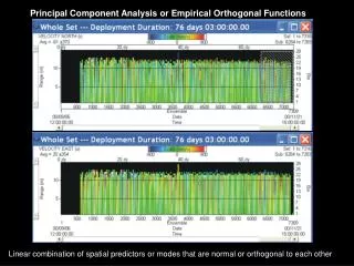
Empirical Orthogonal Functions. Andy Jacobson and Brad Holcombe July 2006. Variance and Covariance. Notes: E() is expectation (mean) M is the number of obs N is the number of stations (locations with data) All vectors are arranged in columns unless transposed.

E N D
Empirical Orthogonal Functions Andy Jacobson and Brad Holcombe July 2006
Variance and Covariance • Notes: • E() is expectation (mean) • M is the number of obs • N is the number of stations (locations with data) • All vectors are arranged in columns unless transposed. • If computing var/cov “by hand”, you must remove the mean of the data at each station. • Degrees of freedom M are reduced by one because of the computation of the mean. • D is the “data matrix” • The spatial dimensions of your input data must be “unwrapped”: 2-D grids must be laid out as a 1-D row in D • C is the covariance matrix.
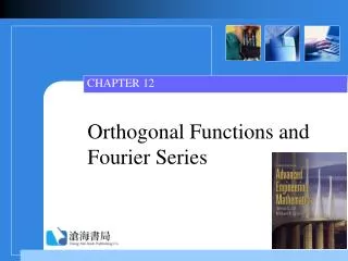
Eigenvalue Decomposition • Two covariate time series, x and y. • Generated from two uncorrelated random number sequences by multiplying by a specified covariance matrix.
Eigenvalue Decomposition • Notes: • C is the covariance matrix • E is the matrix of eigenvectors • is the diagonal matrix of eigenvalues
Eigenvalue Decomposition • Notes: • C is the covariance matrix • E is the matrix of eigenvectors • is the diagonal matrix of eigenvalues
Eigenvalue Decomposition • Notes: • C is the covariance matrix • E is the matrix of eigenvectors • is the diagonal matrix of eigenvalues
Eigenvalue Decomposition • Notes: • C is the covariance matrix • E is the matrix of eigenvectors • is the diagonal matrix of eigenvalues
Eigenvalue Decomposition • Notes: • C is the covariance matrix • E is the matrix of eigenvectors • is the diagonal matrix of eigenvalues
Eigenvalue Decomposition • Notes: • C is the covariance matrix • E is the matrix of eigenvectors • is the diagonal matrix of eigenvalues
Eigenvalue Decomposition • Notes: • C is the covariance matrix • E is the matrix of eigenvectors • is the diagonal matrix of eigenvalues
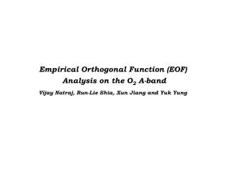
EOFs • Notes: • EOF terminology is not well defined. Conflicting definitions are common in the literature. • The projection of each eigenvector onto the data gives a time series of “scores”. • A is the matrix of score time series and has dimensions M x N • “Principal components” often refers to the scores. • “PCA”, however, is sometimes taken to mean an eigen decomposition of the correlation matrix. • The observations from any given time can be recovered with a weighted sum of the eigenvector scores from that time (row)
EOF Examples Retrieving the magnitude and time series of two static patterns Effects of noise, missing data, and few data Interpretation Propagating features NAO example Exercise: ENSO