Download
1 / 84
840 likes | 958 Views
Automatic Performance Tuning of Numerical Kernels BeBOP: Berkeley Benchmarking and OPtimization. James Demmel EECS and Math UC Berkeley. Katherine Yelick EECS UC Berkeley. Support from NSF, DOE SciDAC, Intel. Performance Tuning Participants. Other Faculty

E N D
Automatic Performance Tuningof Numerical Kernels BeBOP: Berkeley Benchmarking and OPtimization James Demmel EECS and Math UC Berkeley Katherine Yelick EECS UC Berkeley Support from NSF, DOE SciDAC, Intel
Performance Tuning Participants • Other Faculty • Michael Jordan, William Kahan, Zhaojun Bai (UCD) • Researchers • Mark Adams (SNL), David Bailey (LBL), Parry Husbands (LBL), Xiaoye Li (LBL), Lenny Oliker (LBL) • PhD Students • Rich Vuduc, Yozo Hida, Geoff Pike • Undergrads • Brian Gaeke , Jen Hsu, Shoaib Kamil, Suh Kang, Hyun Kim, Gina Lee, Jaeseop Lee, Michael de Lorimier, Jin Moon, Randy Shoopman, Brandon Thompson
Outline • Motivation, History, Related work • Tuning Dense Matrix Operations • Tuning Sparse Matrix Operations • Results on Sun Ultra 1/170 • Recent results on P4 • Recent results on Itanium • Future Work
Performance Tuning • Motivation: performance of many applications dominated by a few kernels • CAD Nonlinear ODEs Nonlinear equations Linear equations Matrix multiply • Matrix-by-matrix or matrix-by-vector • Dense or Sparse • Information retrieval by LSI Compress term-document matrix … Sparse mat-vec multiply • Many other examples (not all linear algebra)
Conventional Performance Tuning • Motivation: performance of many applications dominated by a few kernels • Vendor or user hand tunes kernels • Drawbacks: • Very time consuming and tedious work • Even with intimate knowledge of architecture and compiler, performance hard to predict • Growing list of kernels to tune • Example: New BLAS (Basic Linear Algebra Subroutines) Standard • Must be redone for every architecture, compiler • Compiler technology often lags architecture • Not just a compiler problem: • Best algorithm may depend on input, so some tuning at run-time. • Not all algorithms semantically or mathematically equivalent
Automatic Performance Tuning • Approach: for each kernel • Identify and generate a space of algorithms • Search for the fastest one, by running them • What is a space of algorithms? • Depending on kernel and input, may vary • instruction mix and order • memory access patterns • data structures • mathematical formulation • When do we search? • Once per kernel and architecture • At compile time • At run time • All of the above
Some Automatic Tuning Projects • PHIPAC (www.icsi.berkeley.edu/~bilmes/phipac) (Bilmes,Asanovic,Vuduc,Demmel) • ATLAS (www.netlib.org/atlas) (Dongarra, Whaley; in Matlab) • XBLAS (www.nersc.gov/~xiaoye/XBLAS) (Demmel, X. Li) • Sparsity (www.cs.berkeley.edu/~yelick/sparsity) (Yelick, Im) • FFTs and Signal Processing • FFTW (www.fftw.org) • Won 1999 Wilkinson Prize for Numerical Software • SPIRAL (www.ece.cmu.edu/~spiral) • Extensions to other transforms, DSPs • UHFFT • Extensions to higher dimension, parallelism • Special session at ICCS 2001 • Organized by Yelick and Demmel • www.ucalgary.ca/iccs • Proceedings available • Pointers to other automatic tuning projects at • www.cs.berkeley.edu/~yelick/iccs-tune
Tuning Techniques in PHIPAC • Multi-level tiling (cache, registers) • Copy optimization • Removing false dependencies • Exploiting multiple registers • Minimizing pointer updates • Loop unrolling • Software pipelining • Exposing independent operations • Copy optimization
Untiled (“Naïve”) n x n Matrix Multiply Assume two levels of memory: fast and slow for i = 1 to n {read row i of A into fast memory} for j = 1 to n {read C(i,j) into fast memory} for k = 1 to n {read B(k,j) into fast memory} C(i,j) = C(i,j) + A(i,k) * B(k,j) {write C(i,j) back to slow memory} A(i,:) C(i,j) C(i,j) B(:,j) = + *
Untiled (“Naïve”) n x n Matrix Multiply - Analysis Assume two levels of memory: fast and slow for i = 1 to n {read row i of A into fast memory} for j = 1 to n {read C(i,j) into fast memory} for k = 1 to n {read B(k,j) into fast memory} C(i,j) = C(i,j) + A(i,k) * B(k,j) {write C(i,j) back to slow memory} Count Number of slow memory references m = n3 to read each column of B n times + n2 to read each row of A once for each i + 2n2 to read and write each element of C once = n3 + 3n2
Tiled (Blocked) Matrix Multiply Consider A,B,C to be N by N matrices of b by b subblocks where b=n / N is called the block size for i = 1 to N for j = 1 to N {read block C(i,j) into fast memory} for k = 1 to N {read block A(i,k) into fast memory} {read block B(k,j) into fast memory} C(i,j) = C(i,j) + A(i,k) * B(k,j) {do a matrix multiply on blocks} {write block C(i,j) back to slow memory} A(i,k) C(i,j) C(i,j) = + * B(k,j)
Tiled (Blocked) Matrix Multiply - Analysis • Why is this algorithm correct? • Number of slow memory references on blocked matrix multiply m = N*n2 to read each block of B N3 times (N3 * n/N * n/N) + N*n2 to read each block of A N3 times + 2n2 to read and write each block of C once = (2N + 2) * n2 ~ (2/b) * n3 • b = n/N times fewer slow memory references than untiled algorithm • Assumes all three bxb blocks from A,B,C must fit in fast memory • 3b2 <= M = fast memory size • Decrease in slow memory references limited to a factor of O(sqrt(M)) • Theorem (Hong & Kung, 1981): “Any” reorganization of this algorithm (using only associativity) has at least O(n3/sqrt(M)) slow memory refs • Apply tiling recursively for multiple levels of memory hierarchy
PHIPAC: Copy optimization • Copy input operands • Reduce cache conflicts • Constant array offsets for fixed size blocks • Expose page-level locality Original matrix, column major (numbers are addresses) Reorganized into 2x2 blocks 0 4 8 12 0 2 8 10 1 5 9 13 1 3 9 11 2 6 10 14 4 6 12 13 3 7 11 15 5 7 14 15
PHIPAC: Removing False Dependencies • Using local variables, reorder operations to remove false dependencies a[i] = b[i] + c; a[i+1] = b[i+1] * d; false read-after-write hazard between a[i] and b[i+1] float f1 = b[i]; float f2 = b[i+1]; a[i] = f1 + c; a[i+1] = f2 * d; • With some compilers, you can say explicitly (via flag or pragma) that a and b are not aliased.
PHIPAC: Exploiting Multiple Registers • Reduce demands on memory bandwidth by pre-loading into local variables while( … ) { *res++ = filter[0]*signal[0] + filter[1]*signal[1] + filter[2]*signal[2]; signal++; } Before float f0 = filter[0]; float f1 = filter[1]; float f2 = filter[2]; while( … ) { *res++ = f0*signal[0] + f1*signal[1] + f2*signal[2]; signal++; } also: register float f0 = …; After
PHIPAC: Minimizing Pointer Updates • Replace pointer updates for strided memory addressing with constant array offsets f0 = *r8; r8 += 4; f1 = *r8; r8 += 4; f2 = *r8; r8 += 4; f0 = r8[0]; f1 = r8[4]; f2 = r8[8]; r8 += 12;
PHIPAC: Loop Unrolling • Expose instruction-level parallelism float f0 = filter[0], f1 = filter[1], f2 = filter[2]; float s0 = signal[0], s1 = signal[1], s2 = signal[2]; *res++ = f0*s0 + f1*s1 + f2*s2; do { signal += 3; s0 = signal[0]; res[0] = f0*s1 + f1*s2 + f2*s0; s1 = signal[1]; res[1] = f0*s2 + f1*s0 + f2*s1; s2 = signal[2]; res[2] = f0*s0 + f1*s1 + f2*s2; res += 3; } while( … );
Load(i) Load(i+1) Load(i+2) Mult(i) Mult(i+1) Mult(i+2) Add(i) Add(i+1) Add(i+2) PHIPAC: Software Pipelining of Loops • Mix instructions from different iterations • Keeps functional units “busy” • Reduce stalls from dependent instructions i i+1 i+2 i Load(i+2) Mult(i+1) Add(i) i+1 Load(i+3) Mult(i+2) Add(i+1) Load(i+4) Mult(i+3) Add(i+2) i+2
PHIPAC: Exposing Independent Operations • Hide instruction latency • Use local variables to expose independent operations that can execute in parallel or in a pipelined fashion • Balance the instruction mix (what functional units are available?) f1 = f5 * f9; f2 = f6 + f10; f3 = f7 * f11; f4 = f8 + f12;
Tuning pays off – ATLAS (Dongarra, Whaley) Extends applicability of PHIPAC Incorporated in Matlab (with rest of LAPACK)
Search for optimal register tile sizes on Sun Ultra 10 16 registers, but 2-by-3 tile size fastest
Search for Optimal L0 block size in dense matmul 4% of versions exceed 60% of peak on Pentium II-300
High Precision Algorithms (XBLAS) • Double-double (High precision word represented as pair of doubles) • Many variations on these algorithms; we currently use Bailey’s • Exploiting Extra-wide Registers • Suppose s(1) , … , s(n) have f-bit fractions, SUM has F>f bit fraction • Consider following algorithm for S = Si=1,n s(i) • Sort so that |s(1)| |s(2)| … |s(n)| • SUM = 0, for i = 1 to n SUM = SUM + s(i), end for, sum = SUM • Theorem (D., Hida) Suppose F<2f (less than double precision) • If n 2F-f + 1, then error 1.5 ulps • If n = 2F-f + 2, then error 22f-F ulps (can be 1) • If n 2F-f + 3, then error can be arbitrary (S 0 but sum = 0 ) • Examples • s(i) double (f=53), SUM double extended (F=64) • accurate if n 211 + 1 = 2049 • Dot product of single precision x(i) and y(i) • s(i) = x(i)*y(i) (f=2*24=48), SUM double extended (F=64) • accurate if n 216 + 1 = 65537
Tuning pays off – FFTW (Frigo, Johnson) Tuning ideas applied to signal processing (DFT) Also incorporated in Matlab
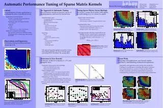
Tuning Sparse matrix-vector multiply • Sparsity • Optimizes y = A*x for a particular sparse A • Im and Yelick • Algorithm space • Different code organization, instruction mixes • Different register blockings (change data structure and fill of A) • Different cache blocking • Different number of columns of x • Different matrix orderings • Software and papers available • www.cs.berkeley.edu/~yelick/sparsity
How Sparsity tunes y = A*x • Register Blocking • Store matrix as dense r x c blocks • Precompute performance in Mflops of dense A*x for various register block sizes r x c • Given A, sample it to estimate Fill if A blocked for varying r x c • Choose r x c to minimize estimated running time Fill/Mflops • Store explicit zeros in dense r x c blocks, unroll • Cache Blocking • Useful when source vector x enormous • Store matrix as sparse 2k x 2l blocks • Search over 2k x 2l cache blocks to find fastest
Register-Blocked Performance of SPMV on Dense Matrices (up to 12x12) 333 MHz Sun Ultra IIi 800 MHz Pentium III 70 Mflops 175 Mflops 35 Mflops 105 Mflops 1.5 GHz Pentium 4 800 MHz Itanium 425 Mflops 250 Mflops 310 Mflops 110 Mflops
Which other sparse operations can we tune? • General matrix-vector multiply A*x • Possibly many vectors x • Symmetric matrix-vector multiply A*x • Solve a triangular system of equations T-1*x • y = AT*A*x • Kernel of Information Retrieval via LSI (SVD) • Same number of memory references as A*x • y = Si (A(i,:))T * (A(i,:) * x) • Future work • A2*x, Ak*x • Kernel of Information Retrieval used by Google • Includes Jacobi, SOR, … • Changes calling algorithm • AT*M*A • Matrix triple product • Used in multigrid solver • What does SciDAC need?
Test Matrices • General Sparse Matrices • Up to n=76K, nnz = 3.21M • From many application areas • 1 – Dense • 2 to 17 - FEM • 18 to 39 - assorted • 41 to 44 – linear programming • 45 - LSI • Symmetric Matrices • Subset of General Matrices • 1 – Dense • 2 to 8 - FEM • 9 to 13 - assorted • Lower Triangular Matrices • Obtained by running SuperLU on subset of General Sparse Matrices • 1 – Dense • 2 – 13 – FEM • Details on test matrices at end of talk