Download

1 / 80
810 likes | 912 Views
Explore Hamiltonian formalism in physics, from Legendre transformations to Hamilton's equations and canonical transformations. Learn how Hamiltonian approach differs from Lagrangian, and its practical utility in various physics fields. Discover how Hamiltonian conserves energy and generates system evolution. Understand higher-derivative Lagrangians and the implications they bring to systems' stability. Uncover the role of canonical transformations and gauge invariance in shaping Hamiltonian dynamics.

E N D
Adrien-Marie Legendre (1752 –1833) • Legendre transformations • Legendre transformation:
What is H? • Conjugate momentum • Then • So
What is H? • If • Then • Kinetic energy • In generalized coordinates
What is H? • For scleronomous generalized coordinates • Then • If
What is H? • For scleronomous generalized coordinates, H is a total mechanical energy of the system (even if H depends explicitly on time) • If H does not depend explicitly on time, it is a constant of motion (even if is not a total mechanical energy) • In all other cases, H is neither a total mechanical energy, nor a constant of motion
Sir William Rowan Hamilton (1805 – 1865) • Hamilton’s equations • Hamiltonian: • Hamilton’s equations of motion:
Hamiltonian formalism • For a system with M degrees of freedom, we have 2M independent variables q and p: 2M-dimensional phase space (vs. configuration space in Lagrangian formalism) • Instead of M second-order differential equations in the Lagrangian formalism we work with 2M first-order differential equations in the Hamiltonian formalism • Hamiltonian approach works best for closed holonomic systems • Hamiltonian approach is particularly useful in quantum mechanics, statistical physics, nonlinear physics, perturbation theory
Hamilton’s equations in symplectic notation • Construct a column matrix (vector) with 2M elements • Then • Construct a 2Mx2M square matrix as follows:
Hamilton’s equations in symplectic notation • Then the equations of motion will look compact in the symplectic (matrix) notation: • Example (M = 2):
Lagrangian to Hamiltonian • Obtain conjugate momenta from a Lagrangian • Write a Hamiltonian • Obtain from • Plug into the Hamiltonian to make it a function of coordinates, momenta, and time
Lagrangian to Hamiltonian • For a Lagrangian quadratic in generalized velocities • Write a symplectic notation: • Then a Hamiltonian • Conjugate momenta
Lagrangian to Hamiltonian • Inverting this equation • Then a Hamiltonian
Hamilton’s equations from the variational principle • Action functional : • Variations in the phase space :
Hamilton’s equations from the variational principle • Integrating by parts
Hamilton’s equations from the variational principle • For arbitrary independent variations
Conservation laws • If a Hamiltonian does not depend on a certain coordinate explicitly (cyclic), the corresponding conjugate momentum is a constant of motion • If a Hamiltonian does not depend on a certain conjugate momentum explicitly (cyclic), the corresponding coordinate is a constant of motion • If a Hamiltonian does not depend on time explicitly, this Hamiltonian is a constant of motion
Higher-derivative Lagrangians • Let us recall: • Lagrangians with i > 1 occur in many systems and theories: • Non-relativistic classical radiating charged particle (see Jackson) • Dirac’s relativistic generalization of that • Nonlinear dynamics • Cosmology • String theory • Etc.
Mikhail Vasilievich Ostrogradsky (1801 - 1862) • Higher-derivative Lagrangians • For simplicity, consider a 1D case: • Variation
Higher-derivative Lagrangians • Generalized coordinates/momenta:
Higher-derivative Lagrangians • Euler-Lagrange equations: • We have formulated a ‘higher-order’ Lagrangian formalism • What kind of behavior does it produce?
Example • H is conserved and it generates evolution – it is a Hamiltonian! • Hamiltonian linear in momentum?!?!?! • No low boundary on the total energy – lack of ground state!!! • Produces ‘runaway’ solutions: the system becomes highly unstable - collapse and explosion at the same time
‘Runaway’ solutions • Unrestricted low boundary of the total energy produces instabilities • Additionally, we generate new degrees of freedom, which require introduction of additional (originally unknown) initial conditions for them • These problems are solved by means of introduction of constraints • Constraints restrict unstable behavior and eliminate unnecessary new degrees of freedom
9.1 • Canonical transformations • Recall gauge invariance (leaves the evolution of the system unchanged): • Let’s combine gauge invariance with Legendre transformation: • K – is the new Hamiltonian (‘Kamiltonian’ ) • K may be functionally different from H
9.1 • Canonical transformations • Multiplying by the time differential: • So
9.1 • Generating functions • Such functions are called generating functions of canonical transformations • They are functions of both the old and the new canonical variables, so establish a link between the two sets • Legendre transformations may yield a variety of other generating functions
9.1 • Generating functions • We have three additional choices: • Canonical transformations may also be produced by a mixture of the four generating functions
9.2 • An example of a canonical transformation • Generalized coordinates are indistinguishable from their conjugate momenta, and the nomenclature for them is arbitrary • Bottom-line: generalized coordinates and their conjugate momenta should be treated equally in the phase space
9.4 • Criterion for canonical transformations • How to make sure this transformation is canonical? • On the other hand • If • Then
9.4 • Criterion for canonical transformations • Similarly, • If • Then
9.4 • Criterion for canonical transformations • So, • If
9.4 • Canonical transformations in a symplectic form • After transformation • On the other hand
9.4 • Canonical transformations in a symplectic form • For the transformations to be canonical: • Hence, the canonicity criterion is: • For the case M = 1, it is reduced to (check yourself)
9.3 • 1D harmonic oscillator • Let us find a conserved canonical momentum • Generating function
9.3 • 1D harmonic oscillator • Nonlinear partial differential equation for F • Let’s try to separate variables • Let’s try
9.3 • 1D harmonic oscillator • We found a generating function!
9.3 1D harmonic oscillator
9.3 1D harmonic oscillator
9.5 • Canonical invariants • What remains invariant after a canonical transformation? • Matrix A is a Jacobian of a space transformation • From calculus, for elementary volumes: • Transformation is canonical if
9.5 • Canonical invariants • For a volume in the phase space • Magnitude of volume in the phase space is invariant with respect to canonical transformations:
9.5 • Canonical invariants • What else remains invariant after canonical transformations?