Download
1 / 50
500 likes | 513 Views
Learn about scientific visualization techniques using MATLAB in this fall 2012 course. Topics include geometry, topology, and data types, scalar and vector visualization, and key resources.

E N D
Scientific Visualization Using MATLAB Robert Putnam putnam@bu.edu Scientific Visualization Using MATLAB - Fall 2012
Outline • Introduction • Geometry / Topology / Data Types • Camera, lights, … • Scalar visualization • Vector visualization • Resources Scientific Visualization Using MATLAB - Fall 2012
Scientific Visualization • Visualization: converting raw data to a form that is viewable and understandable to humans. • Scientific visualization: specifically concerned with data that has a well-defined representation in 2D or 3D space (e.g., from simulation mesh or scanner). *Adaptedfrom The ParaView Tutorial, Moreland Scientific Visualization Using MATLAB - Fall 2012
Generic visualization pipeline Source(s) Filters(s) Output (Rendering) - - - - - - - - - - - - - - - - - - - - - data/geometry/topology graphics Scientific Visualization Using MATLAB - Fall 2012
Geometry v. Topology • Geometry of a dataset ~= points 0,1 1,1 2,1 3,1 0,0 1,0 2,0 3,0 • Topology ~= connections among points, which define cells • So, what’s the topology here? Scientific Visualization Using MATLAB - Fall 2012
Geometry v. Topology 0,1 1,1 2,1 3,1 0,0 1,0 2,0 3,0 Scientific Visualization Using MATLAB - Fall 2012
Geometry v. Topology 0,1 1,1 2,1 3,1 0,0 1,0 2,0 3,0 or 0,1 1,1 2,1 3,1 0,0 1,0 2,0 3,0 Scientific Visualization Using MATLAB - Fall 2012
Geometry v. Topology or 0,1 1,1 2,1 3,1 0,1 1,1 2,1 3,1 0,0 1,0 2,0 3,0 0,0 1,0 2,0 3,0 or 0,1 1,1 2,1 3,1 0,0 1,0 2,0 3,0 Scientific Visualization Using MATLAB - Fall 2012
Geometry v. Topology or 0,1 1,1 2,1 3,1 0,1 1,1 2,1 3,1 0,0 1,0 2,0 3,0 0,0 1,0 2,0 3,0 or or 0,1 1,1 2,1 3,1 0,1 1,1 2,1 3,1 0,0 1,0 2,0 3,0 0,0 1,0 2,0 3,0 Scientific Visualization Using MATLAB - Fall 2012
Geometry/Topology Structure • Structure may be regular or irregular • Regular (structured) • need to store only beginning position, spacing, number of points • smaller memory footprint per cell (topology can be generated on the fly) • examples: image data, rectilinear grid, structured grid • Irregular (unstructured) • information can be represented more densely where it changes quickly • higher memory footprint (topology must be explicitly written) but more freedom • examples: polygonal data, unstructured grid Scientific Visualization Using MATLAB - Fall 2012
Structured Points (Image Data) • regular in both topology and geometry • examples: lines, pixels, voxels • applications: imaging CT, MRI • Rectilinear Grid • regular topology but geometry only partially regular • examples: pixels, voxels • Structured Grid (Curvilinear) • regular topology and irregular geometry • examples: quadrilaterals, hexahedron • applications: fluid flow, heat transfer Examples of Dataset Types Scientific Visualization Using MATLAB - Fall 2012
Examples of Dataset Types (cont) • Polygonal Data • irregular in both topology and geometry • examples: vertices, polyvertices, lines, polylines, polygons, triangle strips • Unstructured Grid • irregular in both topology and geometry • examples: any combination of cells • applications: finite element analysis, structural design, vibration Scientific Visualization Using MATLAB - Fall 2012
Characteristics of Data • Data is organized into datasets for visualization • Datasets consist of two pieces • organizing structure • points (geometry) • cells (topology) • data attributes associated with the structure • Data is discrete • Interpolation functions generate data values in between known points Scientific Visualization Using MATLAB - Fall 2012
MATLAB – Data Types Basic data type • The basic data type is the array. • “Arrays in MATLAB are N-dimensional, with an infinite number of trailing singleton dimensions. Trailing singleton dimensions past the second are not displayed or reported on (e.g., with size). No array has fewer than two dimensions.” • A vector is an Nx1 (or 1XN) array (and a scalar is a 1x1 array): • Array dimensions are generally reported (e.g., by ‘whos’) in “row by column” order (i.e., y by x). Scientific Visualization Using MATLAB - Fall 2012
MATLAB – Data Types Volume Data • Data defined on three-dimensional grids • Two basic types • Scalar volume data • Single data values for each point • Examples: temperature, pressure, density, elevation • Vector volume data • Two or three values for each point (components of a vector) • Magnitude and direction • Examples: velocity, momentum Scientific Visualization Using MATLAB - Fall 2012
Handle graphics, GUIs • “Handle graphics” • Numerical id assigned to figure window and its components • GUI (for menus, sliders, etc.) Scientific Visualization Using MATLAB - Fall 2012
Figure Figure • All graphical output directed to a graphics window called a figure • Separate from the Command Window • Can contain menus, toolbars, user-interface objects, context menus, axes, or any other type of graphics object. Scientific Visualization Using MATLAB - Fall 2012
Handle Graphics Hierarchy • Root object • (computer screen) • Figure object(s) Scientific Visualization Using MATLAB - Fall 2012
Core graphics objects • Core graphics objects • axis (frame, defines coordinate • system) • line • text • rectangle • light • patch (filled polygons) • surface (3D grid of • quadrilaterals) • image (2D representation) Scientific Visualization Using MATLAB - Fall 2012
Code – figure function Command Window f = figure figure creates a new figure object using default property values. It becomes the current figure and is raised above all other figures on the screen until a new figure is either created or called. Many graphics commands create figures, so often there is no need to invoke the ‘figure’ command explicitly. gcf: current figure figure(f): set current figure to f and make visible close all: close all figure windows shg: show graphic window (ESC to return) gca: current axis object Scientific Visualization Using MATLAB - Fall 2012
Exercise – figure property list Command Window:figure1.m f = figure('Name','Test Window','Position',[100 500 350 350],'MenuBar','none') or f = figure set (f, 'Name', 'Test Window') set (f, 'Position', [100 500 350 350]) set (f, 'MenuBar', 'none') Type get(f,’Name’) to see f’s ‘Name’ property, or get(f) to see all properties [or set(f) to see possible values] Tip #1: Use ‘more on’ to keep list from scrolling. Tip #2: Try inspect(f) or plottools(f). Tip #3: See ‘Handle Graphics Property Browser’ in User Guide. Scientific Visualization Using MATLAB - Fall 2012
MATLAB - Viewing Viewing control • One can alter the appearance of a figure by adjusting the camera position, changing the perspective, changing the aspect ratio, etc. • Two primary functions: • Positioning the viewpoint to orient the scene – viewfunction • Setting the aspect ratio and relative axis scaling – axis function Scientific Visualization Using MATLAB - Fall 2012
MATLAB – view function view • The viewpoint is specified by defining azimuth and elevation with respect to the origin: • Azimuth is a polar angle in the x-y plane, with positive angles indicating counterclockwise rotation of the viewpoint from the -y axis. • Elevation is the angle above or below the x-y plane. Scientific Visualization Using MATLAB - Fall 2012
MATLAB – view function (cont.) view • MATLAB automatically selects a viewpoint that is determined by whether the plot is 2-D or 3-D • For 2-D plots, the default is azimuth = 0° and elevation = 90° • For 3-D plots, the default is azimuth = -37.5° and elevation = 30° • view(2) sets the default 2D view, with az = 0, el = 90. • view(3) sets the default 3D view, with az = –37.5, el = 30. • view(az,el) or view([az,el]) set the viewing angle for a 3D view. Scientific Visualization Using MATLAB - Fall 2012
Exercise – view Command Window: view1 samplefig; view([-20 25]); Scientific Visualization Using MATLAB - Fall 2012
Exercise – view Command Window: view1 Figure menu: - Add X,Y labels - Rotate graph* - Examine values with data cursor - Save figure *Tip: after rotating graph, use get(gca, ‘view’) or inspect(gca) to see new azimuth and elevation. Scientific Visualization Using MATLAB - Fall 2012
MATLAB – axis function axis • Adjust the scaling of graph axes. • axis([xminxmaxyminymaxzminzmax]) sets the limits for the x-axis, y-axis and z-axis of the current axis object. • axis vis3d freezes aspect ratio properties to enable rotation of 3-D objects without rescaling. Scientific Visualization Using MATLAB - Fall 2012
Code – axis function Command Window: axis1 samplefig; view([-20 25]); axis([0 30 0 30 -15 15]); % axis auto; axis vis3d; % axis normal; Tip: Note the effect of using axis ‘normal’ instead of ‘vis3d’ Scientific Visualization Using MATLAB - Fall 2012
MATLAB - Lighting Lighting • Enhances the visibility of surface shape and provides a 3D perspective to your visualization. • Several commands enable you to position light sources and adjust the characteristics of lit objects: • light - creates a light object • lighting - selects a light shading (e.g., interpolation) method (e.g., ‘flat’, ‘gouraud’, ‘phong’) • material - sets the specular (mirror-like) reflectance properties of lit objects (e.g., ‘shiny’, ‘dull’, ‘metal’) • camlight - creates or moves a light with respect to the camera position • shading - controls the color shading of surface and patch graphic objects (e.g., ‘flat’, ‘faceted’, ‘interp’) Scientific Visualization Using MATLAB - Fall 2012
Exercise – lighting, material, etc. Command Window:lighting1 samplefig; light; lighting phong; material (‘shiny’); camlight left; shading interp; Try changing lighting, material, shading, etc., using command or function syntax. E.g. material dull; or material(‘dull’); Phong lighting + flat shading? Scientific Visualization Using MATLAB - Fall 2012
MATLAB – Vis Algorithms • Scalar • Matrix to Surface • Slicing • Color Mapping • Contours / Isosurfaces • Vector • Oriented Glyphs • Streamlines Scientific Visualization Using MATLAB - Fall 2012
MATLAB – scalar algorithms Matrix to Surface • A surface is defined by the z-coordinates of points above a rectangular grid in the x-y plane. • formed by joining adjacent points with straight lines. • useful for visualizing large matrices. • surf(X,Y,Z) creates a shaded surface using Z for the color data as well as surface height. X and Y are vectors or matrices defining the x and y components of the surface. Scientific Visualization Using MATLAB - Fall 2012
Exercise – surf, meshgrid, breakpoints, etc. Command Window:surf1 [step through] [X,Y] = meshgrid(-3:0.25:3); Z = peaks(X,Y); s = surf(X,Y,Z); axis([-3 3 -3 3 -10 10]); l = light; lighting phong; h = camlight (‘left’); peaks is a function of two variables, obtained by translating and scaling Gaussian distributions [X,Y] = meshgrid(x,y) duplicates the vectors x and y across the rows and columns respectively of arrays X and Y. (meshgrid(x) is equivalent to meshgrid(x,x)). • Set breakpoint in editor • F5 to start, then C-0 to return to cmd. window • F10 to step • Sh-F5 to exit debugger Scientific Visualization Using MATLAB - Fall 2012
MATLAB – scalar algorithms Slicing • A slice is a cross-section of the dataset. • Any kind of surface can be used to slice the volume. • The simplest technique is to use a plane to define the cutting surface. • slice (X,Y,Z,V,sx,sy,sz) draws slices of the volume V along the X, Y, Z directions in the volume V at the points in the scalars or vectors sx, sy, and sz. X, Y, and Z are 3D arrays specifying the coordinates for V. • The color at each point is determined by interpolation into the volume V using the current colormap. Scientific Visualization Using MATLAB - Fall 2012
Exercise – flow, slice Command Window:slice1 [x,y,z,v] = flow; f = figure; xslice = 5; yslice = 0; zslice = 0; s = slice(x,y,z,v,xslice,yslice,zslice); light; lighting phong; camlight('left'); shading interp; The flow dataset represents the speed profile of a submerged jet within an infinite tank. Tip: try slice_angle to see a diagonal slice, viewedge_middle(v) for custom datatip, or for the adventurous, sliceomatic(v). Scientific Visualization Using MATLAB - Fall 2012
MATLAB – scalar algorithms Color Mapping • Each scalar value in data set is mapped through a lookup table to a specific color. • The color lookup table is called the colormap: • Three-column 2-D matrix • Each row of the matrix defines a single color by specifying three RGB component values in the range of zero to one. • Created with array operations or with one of the several color table generating functions (e.g., jet, hsv, hot, cool, summer, and gray). (Do • ‘doc colormap to see current list.) • colormap() returns the current colormap • colormap(map) sets the colormap to the matrix map. Scientific Visualization Using MATLAB - Fall 2012
Code – colormap function Command Window:colormap1 [x,y,z,v] = flow; xslice = 5; yslice = 0; zslice = 0; s = slice(x,y,z,v,xslice,yslice,zslice); view(3); axis([0 10 -4 4 -3 3]); grid on; colormap (flipud(jet(64))); colorbar('vertical'); shading interp; Pop quiz: how would you reverse the order of the entries in the colormap after running colormap1? Scientific Visualization Using MATLAB - Fall 2012
MATLAB – colormap editor If you want even more control over color mapping, you can use the colormap editor. You can open the colormap editor by selecting Colormap from the figure’s Edit menu. Tip: to view a list of colormaps, click ‘Tools’ For a quick look at the current colormap, try: % imagesc(1:64); Scientific Visualization Using MATLAB - Fall 2012
MATLAB – scalar algorithms Contours / Isosurfaces • Construct a boundary between distinct regions in the data • Contours are lines or surfaces of constant scalar value. • Isolines for two-dimensional data and isosurfaces for three-dimensional data • contour(X,Y,Z,v) draws a contour plot of matrix Z with isolines at the data values specified in the vector v. • isosurface(X,Y,Z,V,isovalue) computes isosurface data from the volume data V at the isosurface value specified in isovalue. The isosurface function connects points to create surfaces that have the specified value. Scientific Visualization Using MATLAB - Fall 2012
Code – contour function Command Window:contour1 [X,Y] = meshgrid(-3:0.25:3); Z = peaks(X,Y); isovalues = (-3.0:0.5:3.0); [C h] = contour(X,Y,Z,isovalues); grid on; Pop quiz: Compare with imagesc(Z) in another figure window. Why are the colors different? Scientific Visualization Using MATLAB - Fall 2012
Ex. – isosurface step-through Command Window:isosurface1 [x,y,z,v] = flow; isovalue = -1; purple = [1.0 0.5 1.0]; i = isosurface(x,y,z,v,isovalue); p = patch(i); isonormals(x,y,z,v,p); set(p,'FaceColor',purple,'EdgeColor','none'); view([-10 40]); grid on; l = light('Position', [-10, -2, 20]); lighting gouraud; patch is the low-level graphics function that creates patch graphics objects. A patch object is one or more filled polygons defined by the coordinates of its vertices. Quiz: how would you change the light color? [Hint: try using ‘inspect’.] Scientific Visualization Using MATLAB - Fall 2012
Interactive data exploration Editor Window:isosurface1 To explore different isosurface values, highlight the ‘-1’ in this line: isovalue = -1; then use the %1.1 button repeatedly to see isosurfaces of successively smaller value. When you’ve gotten to -0.03 or so, rotate the model, then turn on a camlight. *Again, for the adventurous, try sliceomatic(v) and hold down the left mouse button on the colorbar to see a variable isosurface. Scientific Visualization Using MATLAB - Fall 2012
MATLAB – vector algorithms Oriented Glyphs • Draw an oriented, scaled glyph for each vector. • Glyphs are polygonal objects such as cones or arrows. • Orientation and scale of glyph indicate the direction and magnitude of the vector. • Glyphs may be coloredaccording to vector magnitude or some other scalar value. • coneplot(X,Y,Z,U,V,W,Cx,Cy,Cz) plots vectors as cones or arrows. • X, Y, Z define the coordinates for the vector field • U, V, W define the vector field • Cx, Cy, Cz define the location of the cones in the vector field • coneplot(...,'quiver') draws arrows instead of cones. Scientific Visualization Using MATLAB - Fall 2012
Code – coneplot function Command Window:coneplot1 load wind; xmin = min(x(:)); xmax = max(x(:)); ymin = min(y(:)); ymax = max(y(:)); zmin = min(z(:)); zmax = max(z(:)); scale = 4; [cx cy cz] = meshgrid(xmin:10:xmax,ymin:5:ymax,zmin:2:zmax); coneplot(x,y,z,u,v,w,cx,cy,cz,scale,'quiver'); view([-35 60]); grid off; The wind dataset represents air currents over North America. The dataset contains six 3-D arrays: x, y, and z are coordinate arrays which specify the coordinates of each point in the volume and u, v, and w are the vector components for each point in the volume. Scientific Visualization Using MATLAB - Fall 2012
Ex. – improved coneplot Command Window:coneplot# 1. Use ‘cone’ instead of ‘quiver’: coneplot2 2. Use color to indicate windspeed: coneplot3 3. In coneplot4, use +1 button to move up one xy plane at a time by incrementing z value: [cx cy cz] = meshgrid(xmin:2:xmax,ymin:2:ymax,1); Scientific Visualization Using MATLAB - Fall 2012
MATLAB – vector algorithms Streamlines • The path a massless particle would take flowing through a vector field. • Can be used to convey the structure of a field by providing a snapshot of the flow at a given time. • Multiple streamlines can be created to explore interesting features in the field. • Computed via numerical integration (integrating product of velocity and delta T). • streamline(X,Y,Z,U,V,W,startx,starty,startz) draws stream lines from the vector volume data. • X, Y, and Z define the coordinates for the vector field. • U, V, and W define the vector field. • startx, starty, startz define the starting positions of the streamlines. Scientific Visualization Using MATLAB - Fall 2012
Code – streamline function Command Window:streamline1 load wind; xmin = min(x(:)); xmax = max(x(:)); ymin = min(y(:)); ymax = max(y(:)); zmin = min(z(:)); zmax = max(z(:)); purple = [1.0 0.5 1.0]; [sx sy sz] = meshgrid(xmin,ymin:10:ymax,zmin:2:zmax); h = streamline(x,y,z,u,v,w,sx,sy,sz); set(h,'LineWidth',1,'Color',purple); view([-40 50]); grid off; Scientific Visualization Using MATLAB - Fall 2012
Interactive data exploration Command Window:streamline2 Using – 1.0 and + 1.0 to adjust zval, try to find the two funnels. The rotate tool can be helpful when viewing the streamlines. To save the current camera position, use save_camera_struct. Scientific Visualization Using MATLAB - Fall 2012
MATLAB - Resources • IS&T tutorials • Introduction to MATLAB • www.bu.edu/tech/research/training/tutorials/MATLAB/ • Using MATLAB to Visualize Scientific Data www.bu.edu/tech/research/training/tutorials/visualization-with-MATLAB/ • Websites • www.mathworks.com/products/MATLAB/ • www.mathworks.com/access/helpdesk/help/techdoc/index.html • www.mathworks.com/academia/student_center/tutorials • Wiki • http://MATLABwiki.mathworks.com/ Scientific Visualization Using MATLAB - Fall 2012
Questions? • Tutorial survey: • - http://scv.bu.edu/survey/tutorial_evaluation.html Scientific Visualization Using MATLAB - Fall 2012