Download
1 / 46
460 likes | 636 Views
Supply And Demand. Pertemuan - 3 Moh . Sigit Taruna 2009-Pengantar Ekonomi I. The Market Mechanism. The Supply Curve The supply curve shows how much of a good producers are willing to sell at a given price, holding constant other factors that might affect quantity supplied

E N D
Supply And Demand Pertemuan - 3 Moh. SigitTaruna 2009-Pengantar Ekonomi I
The Market Mechanism • The Supply Curve • The supply curve shows how much of a good producers are willing to sell at a given price, holding constant other factors that might affect quantity supplied • This price-quantity relationship can be shown by the equation:
The Market Mechanism • The Demand Curve • The demand curve shows how much of a good consumers are willing to buy as the price per unit changes holding non-price factors constant. • This price-quantity relationship can be shown by the equation:
S The curves intersect at equilibrium, or market- clearing, price. At P0the quantity supplied is equal to the quantity demanded at Q0 . P0 D Q0 The Market Mechanism Price ($ per unit) Quantity
The Market Mechanism A Surplus • The market price is above equilibrium • There is excess supply • Producers lower prices • Quantity demanded increases and quantity supplied decreases • The market continues to adjust until the equilibrium price is reached.
Price ($ per unit) S Surplus P1 Assume the price is P1 , then: 1) Qs : Q2 > Qd : Q1 2) Excess supply is Q1:Q2. 3) Producers lower price. 4) Quantity supplied decreases and quantity demanded increases. 5) Equilibrium at P2Q3 P2 D Quantity Q1 Q3 Q2 The Market Mechanism
The Market Mechanism Shortage • The market price is below equilibrium: • There is a shortage • Producers raise prices • Quantity demanded decreases and quantity supplied increases • The market continues to adjust until the new equilibrium price is reached.
Price ($ per unit) S Assume the price is P2 , then: 1) Qd : Q2 > Qs : Q1 2) Shortage is Q1:Q2. 3) Producers raise price. 4) Quantity supplied increases and quantity demanded decreases. 5) Equilibrium at P3, Q3 P3 P2 Shortage D Quantity Q1 Q3 Q2 The Market Mechanism
Supply and Demand • Non-price Determining Variables of Supply • Costs of Production • Labor • Capital • Raw Materials
S S’ P1 P2 Q0 Q1 Q2 Supply and Demand Change in Supply • The cost of raw materials falls • At P1, produce Q2 • At P2, produce Q1 • Supply curve shifts right to S’ • More produced at any price on S’ than on S P Q
Changes In Market Equilibrium (Supply Curve) • Jika biaya turun, harga (P) dan jumlah (Q) tidak selalu konstan • Akan terjadi perubahan, jika supply curve yang baru mencapai ekuilibrium dengan demand curve • Supply curve akan menggeser, maka harga pasar akan jatuh dan jumlah produksi naik • Maka biaya yang rendah menghasilkan harga yang lebih rendah dan penjualan meningkat.
D S S’ P1 P3 Q1 Q3 Q2 Changes In Market Equilibrium • Raw material prices fall • S shifts to S’ • Surplus @ P1 of Q1, Q2 • Equilibrium @ P3, Q3 P Q
Supply and Demand • Non-price Determining Variables of Demand • Income • Consumer Tastes • Price of Related Goods • Substitutes • Complements
D D’ P2 P1 Q0 Q1 Q2 Supply and Demand Change in Demand • Income Increases • At P1, produce Q2 • At P2, produce Q1 • Demand Curve shifts right • More purchased at any price on D’ than on D P Q
D D’ S P3 P1 Q2 Q1 Q3 Changes In Market Equilibrium • Income Increases • Demand shifts to D1 • Shortage @ P1of Q1, Q2 • Equilibrium @ P3, Q3 P Q
D D’ S S’ P2 P1 Q1 Q2 Changes In Market Equilibrium • Income Increases & raw material prices fall • The increase in D is greater than the increase in S • Equilibrium price and quantity increase to P2, Q2 P Q
Elasticity • Elasticity is a general concept that can be used to quantify the response in one variable when another variable changes. • Seberapa besar perubahan jumlah yang diminta sebagai akibat dari perubahan harga Pertemuan - 6 Moh. SigitTaruna 2009
Permintaan Elastis dan Inelastis • Elastis : bila jumlah yang diminta sangat peka terhadap perubahan harga • Inelastis : bila jumlah yang diminta kurang peka terhadap perubahan harga • Price elastic demand : perubahan harga sebesar 1% menyebabkan perubahan jumlah yang diminta lebih dari 1% • Price inelastic demand :perubahan harga sebesar 1% menyebabkan perubahan jumlah yang diminta kurang dari 1%
Price Elasticity of Demand • A popular measure of elasticity is price elasticity of demand measures how responsive consumers are to changes in the price of a product. • The value of demand elasticity is always negative, but it is stated in absolute terms.
Elasticities of Supply and Demand Other Demand Elasticities • Income elasticity of demand measures the percentage change in quantity demanded resulting from a one percent change in income.
Price Elasticity of Demand PX Elastis Elastis Uniter Inelastis QX MRX
When demand does not respond at all to a change in price, demand is perfectly inelastic. Demand is perfectly elastic when quantity demanded drops to zero at the slightest increase in price. Perfectly Elastic andPerfectly Inelastic Demand Curves
Elasticities of Supply and Demand Elasticities of Supply • Price elasticity of supply measures the percentage change in quantity supplied resulting from a 1 percent change in price. • The elasticity is usually positive because price and quantity supplied are directly related.
Elasticities of Supply and Demand Elasticities of Supply • We can refer to elasticity of supply with respect to interest rates, wage rates, and the cost of raw materials.
Elasticities of Supply and Demand The Market for Wheat • 1981 Supply Curve for Wheat • QS = 1,800 + 240P • 1981 Demand Curve for Wheat • QD = 3,550 - 266P
Elasticities of Supply and Demand The Market for Wheat • Equilibrium: Q S = Q D Chapter 2: The Basics of Supply and Demand Slide 26
Elasticities of Supply and Demand The Market for Wheat Chapter 2: The Basics of Supply and Demand Slide 27
Elasticities of Supply and Demand The Market for Wheat • Assume the price of wheat is $4.00/bushel
Changes in the Market: 1981-1998 The Market for Wheat 1981 1,800 + 240P 3,550 - 266P 1,800+240P = 3,550-266P 506P = 1750 P1981 = $3.46/bushel 1998 1,944 + 207P 3,244 - 283P 1,944+207P = 3,244-283P P1998= $2.65/bushel Supply (Qs) Demand (QD) Equilibrium Price (Qs = QD)
Short-Run Versus Long-Run Elasticities Demand • Price elasticity of demand varies with the amount of time consumers have to respond to a price.
Short-Run Versus Long-Run Elasticities Demand • Most goods and services: • Short-run elasticity is less than long-run elasticity. (e.g. gasoline, Drs.) • Other Goods (durables): • Short-run elasticity is greater than long-run elasticity (e.g. automobiles)
DSR Price People tend to drive smaller and more fuel efficient cars in the long-run DLR Quantity Gasoline: Short-Run andLong-Run Demand Curves Gasoline
DLR Price People may put off immediate consumption, but eventually older cars must be replaced. DSR Quantity Automobiles: Short-Run andLong-Run Demand Curves Automobiles
Short-Run Versus Long-Run Elasticities Supply • Most goods and services: • Long-run price elasticity of supply is greater than short-run price elasticity of supply. • Other Goods (durables, recyclables): • Long-run price elasticity of supply is less than short-run price elasticity of supply
SSR Price SLR Due to limited capacity, firms are limited by output constraints in the short-run. In the long-run, they can expand. Quantity Short-Run Versus Long-Run Elasticities Primary Copper: Short-Run and Long-Run Supply Curves
SLR SSR Price Price increases provide an incentive to convert scrap copper into new supply. In the long-run, this stock of scrap copper begins to fall. Quantity Short-Run Versus Long-Run Elasticities Secondary Copper: Short-Run and Long-Run Supply Curves
S’ S A freeze or drought decreases the supply of coffee P1 P0 Short-Run 1) Supply is completely inelastic 2) Demand is relatively inelastic 3) Very large change in price D Q1 Short-Run Versus Long-Run Elasticities Coffee Price Quantity Q0
S’ S Price P2 P0 Intermediate-Run 1) Supply and demand are more elastic 2) Price falls back to P2. 3) Quantity falls to Q2 D Quantity Q2 Q0 Short-Run Versus Long-Run Elasticities Coffee
Price Long-Run 1) Supply is extremely elastic. 2) Price falls back to P0. 3) Quantity increase to Q0. S P0 D Quantity Q0 Short-Run Versus Long-Run Elasticities Coffee
Understanding and Predicting the Effects of Changing Market Conditions • First, we must learn how to “fit” linear demand and supply curves to market data. • Then we can determine numerically how a change in a variable will cause supply or demand to shift and thereby affect the market price and quantity.
Understanding and Predicting the Effects of Changing Market Conditions • Available Data • Equilibrium Price, P* • Equilibrium Quantity, Q* • Price elasticity of supply, ES, and demand, ED.
Supply: Q = c + dP a/b ED = -bP*/Q* ES = dP*/Q* P* -c/d Demand: Q = a - bP Q* Understanding and Predicting the Effects of Changing Market Conditions Price Quantity
Effects of Government Intervention --Price Controls • If the government decides that the equilibrium price is too high, they may establish a maximum allowable ceiling price.
S If price is regulated to be no higher than Pmax, quantity supplied falls to Q1 and quantity demanded increases to Q2. A shortage results P0 Pmax D Excess demand Q0 Effects of Price Controls Price Quantity
Price Controls andNatural Gas Shortages • In 1954, the federal government began regulating the wellhead price of natural gas. • In 1962, the ceiling prices that were imposed became binding and shortages resulted. • Price controls created an excess demand of 7 trillion cubic feet. • Price regulation was a major component of U.S. energy policy in the 1960s and 1970s, and it continued to influence the natural gas markets in the 1980s.