FEATURE EXTRACTION AND FUSION TECHNIQUES FOR PATCH-BASED FACE RECOGITION

1. FEATURE EXTRACTION AND FUSION TECHNIQUES FOR PATCH-BASED FACE RECOGITION Berkay Topcu Sabancı University, 2009

2. Outline • Introduction • Feature Extraction • Dimensionality Reduction • Normalization Methods • Patch-Based Face Recognition • Patch-Based Methods • Classification: Nearest Neighbor Classification • Feature Fusion • Decision Fusion • Experiments and Results • Databases and Experiment Set-up • Closed Set Identification • Open Set Identification • Verification • Conclusions and Future Work

4. Face Recognition Face Image Feature Extraction Dimensionality Reduction and Normalization Feature / Decision Fusion Classification Closed Set Id. / Open Set Id. / Verification Recognition

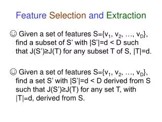
5. Dimensionality Reduction • Feature selection • Dimension reduction • extract relevant structures and relationships • Projecting or mapping d-dimensional data into p-dimensions where p <d • Given d-dimensional data , we want to find p-dimensional data such that :

6. Discrete Cosine Transform (DCT) • Expresses data as summation of cosine functions • Due to its strong energy compaction property, most of the signal information is concantrated in a few low components • Zig-zag scan • First basis : the average intensity • Second and third basis : the average horizontal and vertical intensity change

7. Principal Component Analysis (PCA) • Maps data into a lower dimension by preserving most of its variance • Rows of : eigenvectors that corresponds to the p highest eigenvalues of scatter matrix, • Does not take class information into account, no guarantee for discrimination.

8. Principal Component Analysis (PCA) • 64 x 64 = 4096 pixels/dimensions  192 dimensions First 16 principal components (eigenfaces)

9. Linear Discriminant Analysis (LDA) • Finds the linear combination of features which separate two or more classes • The goal is to maximize between-class scatter while minimizing within-class scatter • Rows of : eigenvectors that corresponds to the p highest eigenvalues of

10. Deficiencies of PCA and LDA • PCA does not take class information into account • LDA faces computational difficulties with large number of highly correlated features, scatter matrices might become singular • When there is less data for each class, scatter matrices are not estimated reliably and there are also numerical problems related to the singularity of scatter matrices • Outlier classes dominate the eigenvalue decomposition, therefore the influence of already well separated classes are overweighted • Distance of already separated classes are preserved, causing overlap of neighboring classes

11. Approximate Pairwise Accuracy Criterion (APAC) • -class LDA can be decomposed into a sum of two-class LDA problems • Contribution of each two-class LDA to the overall criterion is weighted • Rows of : eigenvectors that corresponds to the p highest eigenvalues of • erf : Bayes error of two normal distributed classes

12. Normalized PCA (NPCA) • PCA maximizes the sum of all squared pairwise distances between projected vectors • The idea is to maximize a weighted (pairwise dissimilarities) sum of pairwise distances • Rows of : generalized eigenvectors that corresponds to the p highest eigenvalues of where is a Laplacian matrix derived by pairwise dissimilarities and is data matrix (one sample in each row)

13. Normalized PCA (NPCA)

14. Normalized LDA (NLDA) • Pairwise simillarities are introduced • Aim is to induce “attraction” between elements of the same class and “repulsion” between elements of different classes, by maximizing • Rows of : generalized eigenvectors that corresponds to the p highest eigenvalues of

15. Normalized LDA (NLDA)

16. Nearest Neighbor Discriminant Analysis (NNDA) • Maximizes the distance between classes, while minimizing the expected distance among the samples of same class. where is the sample weight definde as:

17. Nearest Neighbor Discriminant Analysis (NNDA) • Rows of : generalized eigenvectors that corresponds to the p highest eigenvalues of • Extra-class and intra-class differences are calculated in the original space and then projected into low dimensional space, they do not exactly agree with differences in projection space • Stepwise Dimensionality Reduction : In each step, distances are recalculated in its current dimensionality

18. Nearest Neighbor Discriminant Analysis (NNDA)

19. Normalization Methods • Image Domain Mean and Variance Normalization: Aims to exract similar visual feature vectors from each blocks across sessions of same subject.

20. Feature Normalization • Aims to reduce inter-session variability and intra-class variance • Norm Division (ND): • Sample Variance Normalization (SVN): • Block Mean and Variance Normalization (BMVN): • Feature Vector Mean and Variance Normalization (FMVN):

21. Patch-Based Face Recognition • In order to eliminate or lower the effects of illumination changes, occlusion and expression changes by analyzing face images locally • A detected face is divided into blocks of 16x16 or 8x8 pixels size • Dimensionality reduction techniques are applied on each block separately 16x16 blocks 8x8 blocks

22. Patch-Based Face Recognition • Dimension Reduction • 64x64=4096 features  192 features (16x12 or 64x3) • Following feature extraction • Feature Fusion: Concatenate features from each block in order to create visual feature vector of an image • Decision Fusion: Classify each block separately and then combine individual recognition results of each block • Originating point of this study: Global PCA vs. Patch-based PCA

23. Classification Method: Nearest Neighbor Classifier • Why nearest neighbor classification? • Different distance metrics: • Lp-norm between d –dimensional training sample and test sample • Cosine angle between d –dimensional training sample and test sample • In our experiments, we have used L2 –norm but we have also experimented some promising methods with L1–norm and COS

24. Classification Method: Nearest Neighbor Classifier • Distance to class posterior probabilities: • Depends on the distance of to the nearest training sample from each class • After calculating posterior probability for each class, they are normalized by dividing to their summation so that they sum up to 1

25. Feature Fusion • Defining an image in a vector from as where B is the number of blocks and denotes vectorized bthblock of the image, we find a linear tranformation matrix, , such that

26. Decision Fusion • Combining the decisions of each classifier trained by different blocks • Output of a classifier is class posterior probabilities • Fixed combiners • Mean, maximum, minimum, median, sum, product of the set • Majority voting of the individual classifier decisions • Trainable combiners • Use the output of the classifier as a feature set • From class posterior probabilities of several classifiers, a new classifier is trained to provide an ultimate decision

27. Trainable Combiners • Training data is separated as train data and validation data • Stacked generalization

28. Trainable Combiners • Resulting class posterior probabilities are concatenated into a vector as • The length of this input feature vector of the combiner is • In sum rule (fixed combiner) • The posterior probabilities for one class from each classifier are summed. • Weighted summation of posterior probabilities can be performed • Fixed combination method with trainable weights • How to assign weights?

29. Block Weights (Offline Weights) • Learned from training data and independent of test data • Equal Weights (EW): Contribution of each block assumed to be same • Score Weighting (SW): Depends on the posterior probability distribution of true and wrong labels on validation data where and

30. Block Weights (Offline Weights) • (SW continued) LDA finds the linear combination of vectors, such that these vectors are most separated in the projected space. Project 16-dimensional score matrices to 1-dimension and use the coefficients used in this mapping. Negative examples Positive examples

31. Block Weights (Offline Weights) • Validation Accuracy Weighting (VAW): Depends on the individual recognition rates on validation data for each block. However, the most trusted blocks might not contain that much information in a test image due to partial occlusion  a weighting scheme that depends on the training dataset might not be trustworthy and a more interactive scheme that is related with the test sample is believed to provide more accurate weight assignments

32. Confidence Weighting(Online Weighting) • Each test sample is treated separately and individual block weights for each test sample is calculated according to its reliability or confidence • Confidence features are extracted from each block for each sample in the validation data and labeled as “correctly classified” or “misclassified” • Similarity, a measure of closeness of a feature to the mean feature • Block selection • Aims to discard blocks that are not helpful • Blocks are sorted according to block similarity • Selected blocks are weighted according to their confidence weights • The remaining blocks are discarded (their weights are assigned as zero)

33. Experiments and Results - Databases • M2VTS database • 37 subjects – 5 video shots (selected random 8 frames at each video) • 4 tapes for training – 1 tape for testing (includes variations such as different hairstyles, glasses, hats and scarfs) • 32 training images/subject – 8 test images/subject • 1184 (32x37) training images – 296 (8x37) testing images

34. Experiments and Results - Databases • AR database • 120 subjects – two sessions (13 images in each session) • First 7 images of each session  training Remaining 6 images of each session  testing (include sun glasses and scarf – partial occlusion) • 14 training images/subject 12 test images/subject • 1680 training images – 1440 test images

35. Closed Set Identification • Identifying an unknown face if the subject is known to be in the database • Experiments on the M2VTS database • Effect of image domain normalization

36. Experiments on the M2VTS database • Feature Fusion • LDA, APAC, NLDA provide higher recognition accuracies • FMVN increases accuracies, other normalization methods are inconsistent • 16x16 blocks provide higher results than 8x8 blocks • The highest accuracy obtained by NLDA + FMVN : 93.45% • Decision Fusion • DCT and NNDA provide highest recognition accuracies • Image normalization contributes positively (except DCT) • All feature normalization methods are helpful • Baseline is EW and in most cases SW and VAW perform better • The highest accuracies are DCT + ND (VAW) : 97.30% NNDA + SVN (SW) : 96.96%

37. Experiments on the AR database • Feature Fusion • Less data dependent transforms, DCT, PCA, NPCA and NNDA perform well • LDA, APAC and NLDA face problems when there is not enough training data • Image domain normalization is not helpful as train and test data have similar illumination conditions • ND increases accuracies • The highest recognition rate NNDA + ND : 48.08%

38. Experiments on the AR database • Decision Fusion • DCT,PCA and NNDA provide highest recognition accuracies • Image normalization is not helpful • All feature normalization methods are helpful • Baseline is EW and in most cases SW and VAW perform better • The highest accuracies are NNDA + ND (VAW) : 85.97% DCT+ SVN (VAW) : 84.65% • Single training data experiment • To illustrate the effect of normalization methods • By using DCT and EW

39. Confidence Weighting and Block Selection • The weights calculated are close to each other (almost same as EW) • PCA without any normalization methods and EW : 65.49% (AR)

40. Different Distance Metrics • For some of the cases that provide the highest recognition rates

41. Comparison with Other Techniques • CSU Face Identification Evaluation System • PCA, PCA + LDA, Bayesian Intrapersonal/Extrapersonal Difference Classifier • Lining up eye coordinates, masking face, histogram equalization, pixel normalization • Our implemantation of illumination correction + global DCT/global PCA • Our highest accuracies : 97.30% for M2VTS and 89.10% for AR

42. Open Set Identification • There is a rejection option • Determines if the unknown face belongs to the database • Finds the identity of the subject from the database • False Accept Rate (FAR) vs. False Reject Rate + False Classification Rate (FRR+FCR) • M2VTS database, CSI : 97.30% DCT + ND, EER : 14.89%

43. Verification • Confirming or rejecting an unknown face’s claimed identity • FAR vs. FRR • M2VTS database, CSI : 97.30% DCT + ND, EER : 5.74%

44. Conclusion and Future Work • Different dimensionality reduction and normalization techniques for feature fusion and decision fusion methods • Dimensionality reduction methods can be categorized as: DCT, PCA, NPCA, NNDA (less data dependent transforms) and LDA, APAC, NNDA (data dependent transforms) • Patch-based face recognition is superior to global approaches • Decision fusion provides higher recognition results • Contributions: • Recently proposed dimensionality reduction techniques are applied to patch-based face recognition • Image level and feature level normalization methods are introduced • Use of decision fusion techniques for patch-based face recognition is introduced and weights in “weighted sum rule” are estimated using a novel method

45. Conclusion and Future Work • Future Work • Moving block centers so that each block corresponds to same location on the face for all images of all subjects • Using color information in additon to gray scale intensity values • More accurate distance to posterior probability conversion for nearest neighbor classification

46. Thank you ...