Download
1 / 44
440 likes | 658 Views
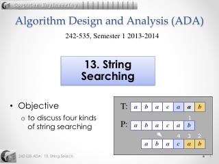
Algorithm Design and Analysis (ADA). 242-535 , Semester 1 2014-2015. Objective describe the quicksort algorithm, it's partition function, and analyse its running time under different data conditions. 5. Quicksort. Overview. Quicksort Partitioning Function Analysis of Quicksort

E N D
Algorithm Design and Analysis (ADA) 242-535, Semester 1 2014-2015 • Objective • describe the quicksort algorithm, it's partition function, and analyse its running time under different data conditions 5. Quicksort
Overview • Quicksort • Partitioning Function • Analysis of Quicksort • Quicksort in Practice
1. Quicksort • Proposed by Tony Hoare in 1962. • Voted one of top 10 algorithms of 20th century in science and engineering • http://www.siam.org/pdf/news/637.pdf • A divide-and-conquer algorithm. • Sorts “in place” -- rearranges elements using only the array, as in insertion sort, but unlike merge sort which uses extra storage. • Very practical (after some code tuning).
Divide and conquer Quicksort an n-element array: 1. Divide: Partition the array into two subarrays around a pivotx such that elements in lower subarray ≤ x ≤ elements in upper subarray. 2. Conquer: Recursively sort the two subarrays. 3. Combine: Nothing to do. Key: implementing a linear-time partitioning function
Pseudocode quicksort(int[] A, int left, int right) if (left < right) // If the array has 2 or more items pivot = partition(A, left, right) // recursively sort elements smaller than the pivot quicksort(A, left, pivot-1) // recursively sort elements bigger than the pivot quicksort(A, pivot+1, right)
Quicksort Diagram pivot
Fine Tuning the Code • quicksort will stop when the subarray is 0 or 1 element big. • When the subarray gets to a small size, switch over to dedicated sorting code rather than relying on recursion. • quicksort is tail-recursive, a recursive behaviour which can be optimized.
Tail-Call Optimization • Tail-call optimization avoids allocating a new stack frame for a called function. • It isn't necesary because the calling function only returns the value that it gets from the called function. • The most common use of this technique is for optimizing tail-recursion • the recursive function can be rewritten to use a constant amount of stack space (instead of linear)
Tail-Call Graphically • Before applying tail-call optimization: • After applying it:
Pseudocode Before: int foo(int n) { if (n == 0) return A(); else { int x = B(n); return foo(x); } } After: int foo(int n) { if (n == 0) return A(); else { int x = B(n); goto start of foo() code with x as argument value } }
2. Partitioning Function PARTITION(A, p, q) // A[p . . q] x ← A[p] // pivot = A[p] Running time i ← p // index = O(n) for n for j ← p + 1 to q elements. if A[ j] ≤ x then i ← i + 1 // move the i boundary exchange A[i] ↔ A[ j] // switch big and small exchange A[p] ↔ A[i] return i // return index of pivot
Example of partitioning scan right until find something less than the pivot
Example of partitioning swap 10 and 5
Example of partitioning resume scan right until find something less than the pivot
Example of partitioning swap 13 and 3
Example of partitioning swap 10 and 2
Example of partitioning j runs to the end
Example of partitioning swap pivot and 2 so in the middle
3. Analysis of Quicksort • The analysis is quite tricky. • Assume all the input elements are distinct • no duplicate values makes this code faster! • there are better partitioning algorithms when duplicate input elements exist (e.g. Hoare's original code) • Let T(n) = worst-case running time on an array of n elements.
3.1. Worst-case of quicksort • QUICKSORT runs very slowly when its input array is already sorted (or is reverse sorted). • almost sorted data is quite common in the real-world • This is caused by the partition using the min (or max) element which means that one side of the partition will have has no elements. Therefore: T(n) = T(0) +T(n-1) + Θ(n) = Θ(1) +T(n-1) + Θ(n) = T(n-1) + Θ(n) = Θ(n2) (arithmetic series) no elements n-1 elements
Worst-case recursion tree T(n) = T(0) +T(n-1) + cn
Worst-case recursion tree T(n) = T(0) +T(n-1) + cn T(n)
Worst-case recursion tree T(n) = T(0) +T(n-1) + cn cn T(0) T(n-1)
Worst-case recursion tree T(n) = T(0) +T(n-1) + cn cn T(0) c(n-1) T(0) T(n-2)
Worst-case recursion tree T(n) = T(0) +T(n-1) + cn cn T(0) c(n-1) T(0) T(n-2) T(0) Θ(1)
Worst-case recursion tree T(n) = T(0) +T(n-1) + cn
Quicksort isn't Quick? • In the worst case, quicksort isn't any quicker than insertion sort. • So why bother with quicksort? • It's average case running time is very good, as we'll see.
3.2. Best-case Analysis If we’re lucky, PARTITION splits the array evenly: T(n) = 2T(n/2) + Θ(n) = Θ(n log n) (same as merge sort) Case 2 of the Master Method
3.3. Almost Best-case What if the split is always 1/10 : 9/10? T(n) = T(1/10n) + T(9/10n) + Θ(n)
Analysis of “almost-best” case cn T(1/10n) T(9/10n)
Analysis of “almost-best” case cn T(1/10n) T(9/10n) T(1/100n ) T(9/100n) T(9/100n) T(81/100n)
Analysis of “almost-best” case short path long path cn * short path cn * long path all leaves
Short and Long Path Heights • Short path node value: n (1/10)n (1/10)2n ... 1 • n(1/10)sp = 1 • n = 10sp // take logs • log10n = sp • Long path node value: n (9/10)n (9/10)2n ... 1 • n(9/10)lp= 1 • n = (10/9)lp // take logs • log10/9n = lp sp steps lp steps
3.4. Good and Bad Suppose we alternate good, bad, good, bad, good, partitions …. G(n) = 2B(n/2) + Θ(n) good B(n) = L(n – 1) + Θ(n) bad Solving: G(n) = 2(G(n/2 – 1) + Θ(n/2) ) + Θ(n) = 2G(n/2 – 1) + Θ(n) = Θ(n log n) How can we make sure we choose good partitions? Good!
Randomized Quicksort IDEA: Partition around a random element. • Running time is then independentof the input order. • No assumptions need to be made about the input distribution. • No specific input leads to the worst-case behavior. • The worst case is determined only by the output of a random-number generator.
4. Quicksort in Practice • Quicksort is a great general-purpose sorting algorithm. • especially with a randomized pivot • Quicksort can benefit substantially from code tuning • Quicksort can be over twice as fast as merge sort • Quicksort behaves well even with caching and virtual memory.
Timing Comparisons • Running time estimates: • Home PC executes 108 compares/second. • Supercomputer executes 1012 compares/second Lesson 1. Good algorithms are better than supercomputers. Lesson 2. Great algorithms are better than good ones.