Download
1 / 105
1.05k likes | 1.07k Views
Learn the efficient Quicksort algorithm, including its partition process and recursive calls, through visual examples and detailed explanations. Explore CS 321 Data Structures concepts.

E N D
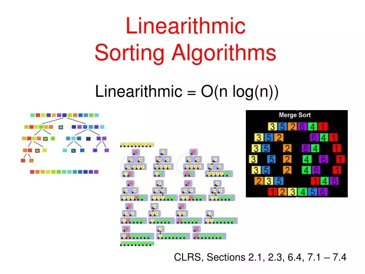
Linearithmic Sorting Algorithms Linearithmic = O(n log(n)) CLRS, Sections 2.1, 2.3, 6.4, 7.1 – 7.4
Linearithmic Sorts • Divide and Conquer Algorithms • Quicksort • Merge Sort • Data Structure Based • Heapsort CS 321 - Data Structures
Quicksort • Quicksort is the most popular, fast sorting algorithm: • It has an average running time case of Θ(n*logn) • The other fast sorting algorithms, Mergesort and Heapsort, also run in Θ(n*logn) time, but • have fairly large constants hidden in their algorithms. • tend to move data around more than desirable. CS 321 - Data Structures
Quicksort • Invented by C.A.R. (Tony) Hoare • A Divide-and-Conquer approach that uses recursion: • If the list has 0 or 1 elements, it’s sorted • Otherwise, pick any element p in the list. This is called the pivot value • Partition the list, minus the pivot, into two sub-lists: • one of values less than the pivot and another of those greater than the pivot • equal values go to either • Return the Quicksort of the first list followed by the Quicksort of the second list. CS 321 - Data Structures
Quicksort Tree Use binary tree to represent the execution of Quicksort • Each node represents a recursive call of Quicksort • Stores • Unsorted sequence before the execution and its pivot • Sorted sequence at the end of the execution • The leaves are calls on sub-sequences of size 0 or 1 9 7 2 4 62 4 6 7 9 2 42 4 9 77 9 2 2 - - 9 9 CS 321 - Data Structures
Example: Quicksort Execution • Pivot selection – last value in list: 6 7 9 4 3 7 1 2 6 - CS 321 - Data Structures
Example: Quicksort Execution • Partition around 6 • Recursive call on sub-list with smaller values 7 9 4 3 7 1 2 6 - 4 3 1 2 - 7 9 7 - CS 321 - Data Structures
Example: Quicksort Execution • Partition around 2 • Recursive call on sub-list of smaller values 7 9 4 3 7 1 2 6 - 4 3 1 2 - 7 9 7 - 1 - 4 3 - CS 321 - Data Structures
Example: Quicksort Execution • Base case • Return from sub-list of smaller values 7 9 4 3 7 1 2 6 - 4 3 1 2 1 2 7 9 7 - 4 3 - 11 CS 321 - Data Structures
Example: Quicksort Execution • Recursive call on sub-list of larger values 7 9 4 3 7 1 2 6 - 4 3 1 2 1 2 7 9 7 - 11 4 3 - CS 321 - Data Structures
Example: Quicksort Execution • Partition around 4 • Recursive call on sub-list of smaller values 7 9 4 3 7 1 2 6 - 4 3 1 2 1 2 7 9 7 - 11 4 3 - - 4 - CS 321 - Data Structures
Example: Quicksort Execution • Base case • Return from sub-list of smaller values 7 9 4 3 7 1 2 6 - 4 3 1 2 1 2 7 9 7 - 11 4 334 - 4 - CS 321 - Data Structures
Example: Quicksort Execution • Recursive call on sub-list of larger values 7 9 4 3 7 1 2 6 - 4 3 1 2 1 2 7 9 7 - 11 4 334 - 4 - CS 321 - Data Structures
Example: Quicksort Execution • Base case • Return from sub-list of larger values 7 9 4 3 7 1 2 6 - 4 3 1 2 1 2 7 9 7 - 11 4 334 - 4 4 CS 321 - Data Structures
Example: Quicksort Execution • Return from sub-list of larger values 7 9 4 3 7 1 2 6 - 4 3 1 2 1 2 3 4 7 9 7 - 11 4 334 - 4 4 CS 321 - Data Structures
Example: Quicksort Execution • Return from sub-list of smaller values 7 9 4 3 7 1 2 61 2 3 4 6 4 3 1 2 1 2 3 4 7 9 7 - 11 4 334 - 4 4 CS 321 - Data Structures
Example: Quicksort Execution • Recursive call on sub-list of larger values 7 9 4 3 7 1 2 61 2 3 4 6 4 3 1 2 1 2 3 4 7 9 7 - 11 4 334 - 4 4 CS 321 - Data Structures
Example: Quicksort Execution • Partition around 7 • Recursive call on sub-list of smaller values 7 9 4 3 7 1 2 61 2 3 4 6 4 3 1 2 1 2 3 4 7 9 7 - 11 4 334 7 - 9 - - 4 4 CS 321 - Data Structures
Example: Quicksort Execution • Base case • Return from sub-list of smaller values 7 9 4 3 7 1 2 61 2 3 4 6 4 3 1 2 1 2 3 4 7 9 7 77 11 4 334 7 7 9 - - 4 4 CS 321 - Data Structures
Example: Quicksort Execution • Recursive call on sub-list of larger values 7 9 4 3 7 1 2 61 2 3 4 6 4 3 1 2 1 2 3 4 7 9 7 77 11 4 334 7 7 9 - - 4 4 CS 321 - Data Structures
Example: Quicksort Execution • Base case • Return from sub-list of larger values 7 9 4 3 7 1 2 61 2 3 4 6 4 3 1 2 1 2 3 4 7 9 7 77 9 11 4 334 7 7 9 9 - 4 4 CS 321 - Data Structures
Example: Quicksort Execution • Return from sub-list of larger values 7 9 4 3 7 1 2 61 2 3 4 6 7 7 9 4 3 1 2 1 2 3 4 7 9 7 77 9 11 4 334 7 7 9 9 - 4 4 CS 321 - Data Structures
Example: Quicksort Execution • Done 7 9 4 3 7 1 2 61 2 3 4 6 7 7 9 4 3 1 2 1 2 3 4 7 9 7 77 9 11 4 334 7 7 9 9 - 4 4 CS 321 - Data Structures
Quicksort Algorithm // A: array of values // p: beginning index of sub-list being sorted // r: ending index of sub-list being sorted // Initial call: Quicksort(A, 1, A.length) CS 321 - Data Structures
Quicksort Partition Algorithm CS 321 - Data Structures
Example: Quicksort Partition Partition(A, 1, A.length) x = A[7] = 6 i = p - 1 = 0 j = 1 A[1] = 2 ≤ 6 i = 0 + 1 = 1 swap A[1], A[1] CS 321 - Data Structures
Example: Quicksort Partition Partition(A, 1, A.length) j = 2 A[2] = 8 > 6 no change CS 321 - Data Structures
Example: Quicksort Partition Partition(A, 1, A.length) j = 3 A[3] = 7 > 6 no change CS 321 - Data Structures
Example: Quicksort Partition Partition(A, 1, A.length) j = 4 A[4] = 1 ≤ 6 i = 1 + 1 = 2 swap A[2], A[4] CS 321 - Data Structures
Example: Quicksort Partition Partition(A, 1, A.length) j = 5 A[5] = 3 ≤ 6 i = 2 + 1 = 3 swap A[3], A[5] CS 321 - Data Structures
Example: Quicksort Partition Partition(A, 1, A.length) j = 6 A[6] = 5 ≤ 6 i = 3 + 1 = 4 swap A[4], A[6] CS 321 - Data Structures
Example: Quicksort Partition Partition(A, 1, A.length) j = 7 for loop done swap A[5], A[7] return 5 CS 321 - Data Structures
Example: Quicksort Partition Partition(A, 1, A.length) Partition complete CS 321 - Data Structures
Runtime Analysis: Best Case • What is best case running time? • Assume keys are random, uniformly distributed. • Recursion: • Partition splits list in two sub-lists of size: (n/2) • Quicksort each sub-list. • Depth of recursion tree? O(logn) • Number of accesses in partition? O(n) • Best case running time: O(n*logn) CS 321 - Data Structures
Runtime Analysis: Worst Case • What is worst case running time? • List already sorted. • Recursion: • Partition splits array in two sub-arrays: • one sub-array of size: 0 • the other sub-array of size: n-1 • Quicksort each sub-array. • Depth of recursion tree? O(n) • Number of accesses per partition? O(n) • Worst case running time: O(n2) CS 321 - Data Structures
Average Case for Quicksort • If the list is already sorted, Quicksort is terrible: O(n2) • It is possible to construct other bad cases. • However, Quicksort is usuallyO(n*logn) • Because the constants are so good, Quicksort is generally the fastest known, comparison-based algorithm. • Most real-world sorting is done by Quicksort. CS 321 - Data Structures
Tweaking Quicksort • Almost anything you can try to “improve” Quicksort will actually slow it down. • One good tweak is to switch to a different sorting method when the subarrays get small (say, 10 or 12). • Quicksort has too much overhead for small array sizes. • For large arrays, it might be a good idea to check beforehand if the array is already sorted. • But there is a better tweak than this. CS 321 - Data Structures
Picking a Better Pivot • Before, we picked the first element of the sub-list to use as a pivot. • If the array is already sorted, this results in O(n2) behavior. • It’s no better if we pick the last element. • We could do an optimal Quicksort if we always picked a pivot value that exactly cuts array in half. • Such a value is called a median: half of the values in the list are larger, half are smaller. • The easiest way to find the median is to sort the list and pick the value in the middle. (!) CS 321 - Data Structures
Median of Three • Obviously, it doesn’t make sense to sort list in order to find median. • Instead, compare just three elements of sub-list: first, last, and middle. • Take the median (middle value) of these three as pivot. • If rearrange (sort) these three numbers so that the smallest is in the first position, the largest in the last position, and the other in the middle. • Simplifies and speeds up the partition loop. CS 321 - Data Structures
Mergesort Algorithm • If a list has 1 element or 0 elements, it’s sorted. • If a list has more than 1, split into two separate lists. • Perform this algorithm on each of those smaller lists. • Take the 2 sorted lists and merge them together. Don Knuth cites John von Neumann as the creatorof this algorithm: CS 321 - Data Structures
Mergesort When implementing, one temporary array is used instead of multiple temporary arrays. Why? CS 321 - Data Structures
Mergesort Tree Use binary tree to represent the execution of Mergesort • Each node represents a recursive call of Mergesort. • Stores • Unsorted sequence before the execution and its pivot. • Sorted sequence at the end of the execution. • The leaves are calls on sub-sequences of size 0 or 1. 7 2 9 4 2 4 7 9 7 2 2 7 9 4 4 9 2 2 9 9 7 7 4 4 CS 321 - Data Structures
Example: Mergesort Execution • List to be sorted 5 9 4 3 7 1 2 6 - CS 321 - Data Structures
Example: Mergesort Execution • Divide values in half between 3 and 7. 5 9 4 3/7 1 2 6 - CS 321 - Data Structures
Example: Mergesort Execution • Recursive call on first sub-list. 5 9 4 3 7 1 2 6 - 5 9 4 3 - 7 1 2 6 - CS 321 - Data Structures
Example: Mergesort Execution • Divide values in half between 9 and 4. 5 9 4 3 7 1 2 6 - 5 9/4 3 - 7 1 2 6 - CS 321 - Data Structures
Example: Mergesort Execution • Recursive call on first sub-list. 5 9 4 3 7 1 2 6 - 5 94 3 - 7 1 2 6 - 5 9 - 4 3 - CS 321 - Data Structures
Example: Mergesort Execution • Divide values in half between 5 and 9. 5 9 4 3 7 1 2 6 - 5 9 4 3 - 7 1 2 6 - 5/9 - 4 3 - CS 321 - Data Structures
Example: Mergesort Execution • Recursive call on first sub-list. 5 9 4 3 7 1 2 6 - 5 9 4 3 - 7 1 2 6 - 5 9 - 4 3 - 5 - 9 - CS 321 - Data Structures
Example: Mergesort Execution • Base case. • First sub-list returns 5. 5 9 4 3 7 1 2 6 - 5 9 4 3 - 7 1 2 6 - 5 9 - 4 3 - 55 9 - CS 321 - Data Structures