Download
1 / 28
280 likes | 669 Views
k-space Data Pre-processing for Artifact Reduction in MRI. SK Patch UW-Milwaukee. thanks KF King, L Estkowski, S Rand for comments on presentation A Gaddipatti and M Hartley for collaboration on Propeller productization. . 660Hz. 392Hz. G. E. C. 523.2Hz. pitch/frequency.

E N D
k-space Data Pre-processing for Artifact Reduction in MRI SK Patch UW-Milwaukee thanks KF King, L Estkowski, S Rand for comments on presentation A Gaddipatti and M Hartley for collaboration on Propeller productization.
660Hz 392Hz G E C 523.2Hz pitch/frequency temporal frequency time pitch/frequency
apodized reconstructed image. checkerboard pattern strong k-space signal along axes log of k-space magnitude data.
Heisenberg Functions cannot be space- and band-limited. implies Riemann-Lebesgue k-space data decays with frequency Heisenberg, Riemann & Lebesgue
Ringing near the edge of a disc. Solid line for k-space data sampled on 512x512; dashed for 128x128; dashed-dot on 64x64 grid. Cartesian sampling reconstruct directly with Fast Fourier Transform (FFT)
spirals – fast acquisition From Handbook of MRI Pulse Sequences. Propeller – redundant data permits motion correction. non-Cartesian sampling requires gridding additional errors
CT errors high-frequency & localized MR errors low-frequency & global CT vs. MRI
linear interpolation = convolve w/“tent” function “gridding” = convolve w/kernel (typically smooth, w/small support) naive k-space gridding low-order interp smooths corrected for gridding errors high-order interp overshoots
sinc interp in k-space 2x Field-of-View convolution – properties Avoid Aliasing Artifacts
Avoid Aliasing Artifacts Propeller k-space data interpolated onto 4x fine grid
sinc interp convolution – properties Image Space Upsampling
Image Space Upsampling sinc-interpolated up to 64x512. image from a phase corrected Propeller blade with ETL=36 and readout length=320.
k-space apodization Reprinted with permission from Handbook of MRI Pulse Sequences. Elsevier, 2004. PSF in image space. Tukey window function in k-space Ringing near the edge of a disc. Solid line for k-space data sampled on 512x512; dashed for 128x128; dashed-dot on 64x64 grid.
high-order interp overshoots w/o gridding deconvolution after gridding deconv cubic interp cubic interp linear interp linear interp no interpolation no shading k-space data sampled at ‘X’s and linearly interpolated onto ‘’s. Low-frequency Gridding Errors no interpolation-no shading; interpolation onto Dk/4 lattice 4xFOV linear interpolation “tent” function against which k-space data is convolved
sinc interp Cartesian sampling suited to sinc-interpolation
Radial sampling (PR, spiral, Propeller) suited to jinc-interpolation
perfect jinc kernel “fast” conv kernel 64 256 multiply image
Propeller – Phase Correct Redundant data must agree, remove phase from each blade image
CORRECTED Propeller – Phase Correct one blade RAW
w/motion correction artifacts due to blade #1 errors sans motion correction Propeller - Motion Correct 2 scans – sans motion
blade #1 Propeller – Blade Correlation throw out bad – or difficult to interpret - data Propeller – Blade Correlation throw out bad – or difficult to interpolate - data blade weights rotations in degrees 1 blade # 23 shifts in pixels
Fourier Transform Properties shift image phase roll across data b is blade image, r is reference image
No correction, with correction shifts in pixels max at Dx
“holes” in k-space Fourier Transform Properties rotate imagerotate data
correlation correction only motion correction only full corrections no correction
Backup Slides Simulations show Cartesian acquisitions are robust to field inhomogeneity. (top left) Field inhomogeneity translates and distorts k-space sampling more coherently than in spiral scans. (top right) magnitude image suffers fewer artifacts than spiral, despite (bottom left) severe phase roll. (bottom right) Image distortion displayed in difference image between magnitude images with and without field inhomogeneity. k-space stretching decreases the field-of-view (FOV), essentially stretching the imaging object.
Backup Slides Propeller blades sample at points denoted with ‘o’ and are upsampled via sinc interpolation to the points denoted with ‘’