Download
1 / 9
90 likes | 183 Views
Range Spectroscopy A review of chop-nod and Unchopped results. Phil Appleton based on material from a study by Roland Vavrek (ESAC). Apparent “Fringing” but in reality “aliasing” (beating) between large grating steps and 16 “spectral” pixels. High Frequency “Noise” due to aliasing.

E N D
Range Spectroscopy A review of chop-nod and Unchopped results Phil Appleton based on material from a study by Roland Vavrek (ESAC)
Apparent “Fringing” but in reality “aliasing” (beating) between large grating steps and 16 “spectral” pixels High Frequency “Noise” due to aliasing
The problem can be solved if the response between adjacent spectral pixels can be normalized (a kind of second-order rsrf). Fit a smooth function (spline or something like it) to each spectral pixel along time dimension (== scan up and down) and use this to adjust the response from one spectral pixel to the next. This removes the periodic jumps. It is a kind of low- pass filter applied to each spectral pixel. The 16 curves are then normalized to the mean of the means.
NEPTUNE B2A Filter (“Green” 2nd order) Before correction After correction
NEPTUNE B2A Filter (“Green” 2nd order) Zoomed in shows even better behavior in corrected spectrum Before After Spectrum totally dominated by the aliasing effect Huge increase in S/N ratio
RANGE CHOP NOD SPECTRUM Zoom even further shows that some residuals still remain but significant improvement
This correction is now incorporated into the standard chop-nod pipeline # Refine the spectral flatfield. # Parameters: # minWaveRangeForPoly (microns). If your spectral ranges are > this value, a poly is fit to the # spectra, of order "polyOrder", on a pixel by pixel basis independently for each module/spaxel. # This (continuum) fit is then used normalise the individual 16 pixels to the module/spaxel mean. # minWaveRangeForPoly (microns). If your spectral ranges are < this values, the median of the spectra, # is calculated, on a pixel by pixel basis independently for each module/spaxel. # This value is then used normalise the individual pixels to the module/spaxel median. # --> the values of polyOrder and minWaveRangeForPoly can be adjusted by the user # In both cases the correction is a division. # # See also the specFlatFieldRange URM entry and the PDRG Chap. 3 for more information. slicedFrames = specFlatFieldRange(slicedFrames,polyOrder=5, minWaveRangeForPoly=4., verbose=1, doPlot=1) provides plots of the ployfit to each spectral pixel to assess quality of fitting http://www.herschel.be/twiki/bin/view/Public/PacsDocumentation http://www.herschel.be/twiki/pub/Public/PacsDocumentation/PDRG_Jan2011.pdf for more details on DATA REDUCTION updates Jan 2011 page 34 describes task
CHOPPED (RED) VERSUS UNCHOPPED (BLACK) FOR SAMESPECTRAL RANGE AND WITH CORRECTION APPLIED Note excellent baselines for Unchopped but 20-30% variations in continuum Unchopped mode is not a good one if you want to reproduce the continuum accurately. Other issues remain (see talk tomorrow on large-range scans.
Conclusions • Corrections to “second-order” rsrf reduces fringing effects significantly • Unchopped mode seems to produce very stable baselines but although line fluxes are reliable, the continuum is very unrelieable. However, as we shall see tomorrow, the chop-nod mode also has large-scale rsrf-type ripples that lead to problems. -- One solution will be discussed tomorrow—using the bright telescope emission as a spectral reference


![Reversing Malware [based on material from the textbook]](https://cdn2.slideserve.com/4174046/reversing-malware-based-on-material-from-the-textbook-dt.jpg)