Lattice Design Theory and Backward Analyses

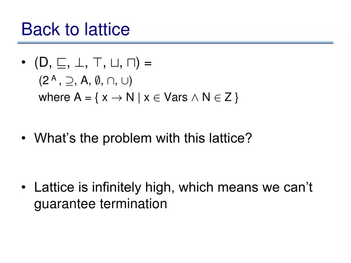
1. Back to lattice • (D, v, ?, >, t, u) = (2 A , ¶, A, ;, Å, [) where A = { x ! N | x 2 Vars Æ N 2 Z } • What’s the problem with this lattice? • Lattice is infinitely high, which means we can’t guarantee termination

2. Better lattice • Suppose we only had one variable

3. Better lattice • Suppose we only had one variable • D = {?, > } [ Z • 8 i 2 Z . ?v i Æ i v> • height = 3

4. For all variables • Two possibilities • Option 1: Tuple of lattices • Given lattices (D1, v1, ?1, >1, t1, u1) ... (Dn, vn, ?n, >n, tn, un) create: tuple lattice Dn =

5. For all variables • Two possibilities • Option 1: Tuple of lattices • Given lattices (D1, v1, ?1, >1, t1, u1) ... (Dn, vn, ?n, >n, tn, un) create: tuple lattice Dn = ((D1£ ... £ Dn), v, ?, >, t, u) where ? = (?1, ..., ?n) > = (>1, ..., >n) (a1, ..., an) t (b1, ..., bn) = (a1t1 b1, ..., antn bn) (a1, ..., an) u (b1, ..., bn) = (a1u1 b1, ..., anun bn) height = height(D1) + ... + height(Dn)

6. For all variables • Option 2: Map from variables to single lattice • Given lattice (D, v1, ?1, >1, t1, u1) and a set V, create: map lattice V ! D = (V ! D, v, ?, >, t, u)

7. Back to example in Fx := y op z(in) = x := y op z out

8. Back to example in Fx := y op z(in) = in [ x ! in(y) op in(z) ] where a op b = x := y op z out

9. General approach to domain design • Simple lattices: • boolean logic lattice • powerset lattice • incomparable set: set of incomparable values, plus top and bottom (eg const prop lattice) • two point lattice: just top and bottom • Use combinators to create more complicated lattices • tuple lattice constructor • map lattice constructor

10. May vs Must • Has to do with definition of computed info • Set of x ! y must-point-to pairs • if we compute x ! y, then, then during program execution, x must point to y • Set of x! y may-point-to pairs • if during program execution, it is possible for x to point to y, then we must compute x ! y

11. May vs must

12. May vs must

13. Direction of analysis • Although constraints are not directional, flow functions are • All flow functions we have seen so far are in the forward direction • In some cases, the constraints are of the form in = F(out) • These are called backward problems. • Example: live variables • compute the set of variables that may be live

14. Example: live variables • Set D = • Lattice: (D, v, ?, >, t, u) =

15. Example: live variables • Set D = 2 Vars • Lattice: (D, v, ?, >, t, u) = (2Vars, µ, ; ,Vars, [, Å) in Fx := y op z(out) = x := y op z out

16. Example: live variables • Set D = 2 Vars • Lattice: (D, v, ?, >, t, u) = (2Vars, µ, ; ,Vars, [, Å) in Fx := y op z(out) = out – { x } [ { y, z} x := y op z out

17. Example: live variables x := 5 y := x + 2 y := x + 10 x := x + 1 ... y ...

18. Example: live variables x := 5 y := x + 2 y := x + 10 x := x + 1 ... y ... How can we remove the x := x + 1 stmt?

19. Revisiting assignment in Fx := y op z(out) = out – { x } [ { y, z} x := y op z out

20. Revisiting assignment in Fx := y op z(out) = out – { x } [ { y, z} x := y op z out

21. Theory of backward analyses • Can formalize backward analyses in two ways • Option 1: reverse flow graph, and then run forward problem • Option 2: re-develop the theory, but in the backward direction