Download
1 / 16
160 likes | 178 Views
This study compares full-band Monte Carlo and Non-equilibrium Green’s Function simulations for advanced modeling of nanoscale device transport. The research focuses on quantum coherence, tunneling behavior, and includes quantum corrections and sub-band details. The collaboration between the University of Illinois and Purdue University explores the strengths and limitations of both simulation techniques, emphasizing the physical details and computational costs. By analyzing a 2-D double-gate MOSFET model with various device parameters, the benchmark comparison highlights agreement and discrepancies between the two approaches, particularly in potential and density profiles under different bias conditions. The study sheds light on the effectiveness and limits of quantum correction potential approaches in Monte Carlo simulations and the velocity overshoot phenomenon observed in Non-equilibrium Green’s Function simulations at high fields.

E N D
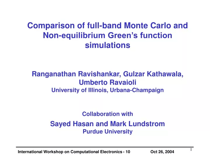
Comparison of full-band Monte Carlo and Non-equilibrium Green’s function simulations Ranganathan Ravishankar, Gulzar Kathawala, Umberto Ravaioli University of Illinois, Urbana-Champaign Collaboration with Sayed Hasan and Mark Lundstrom Purdue University
strengths: - advanced scattering models - band structure readily included - moderate computational cost • strengths: • - quantum coherence • tunneling and evanescent • behavior at barriers Semi-classical transport Ballistic quantum transport particle wave inclusion of: - quantum corrections - quantum sub-band details inclusion of: - scattering models - band structure details Motivation • There is still a considerable separation between semi-classical and quantum models in terms of physical detail
tox S D tSI tox S1 S1 u LG u LT Benchmark Model • We have considered a 2-D device model for the double-gate MOSFET performing simulations with MOCA 2-D (UIUC) NanoMOS (Purdue). Device parameters tox = 1.0 nm ( k = 1.0 ) tSi = 4.0 nm, 3.0 nm, 2.0 nm S1 = 6.0 nm u = underlap = 4.0 nm LG = 9.0 nm (-4.5nm to 4.5nm) LT = 17.0 nm (-8.5nm to 8.5nm) NS/D = 1020 cm-3 (gradient 1.0 nm/decade) Nbody = 1010 cm-3
tSi = 4nm, Vds = 0.05V, Vg = 0.05V tSi = 4nm, Vds = 0.05V, Vg = 0.20V
tSi = 4nm, Vds = 0.05V, Vg = 0.35V tSi = 4nm, Vds = 0.05V, Vg = 0.50V
tSi = 4nm, Vds = 0.20V, Vg = 0.35V tSi = 4nm, Vds = 0.20V, Vg = 0.50V
tSi = 4nm, Vds = 0.35V, Vg = 0.35V tSi = 4nm, Vds = 0.35V, Vg = 0.50V
tSi = 4nm, Vds = 0.50V, Vg = 0.35V tSi = 4nm, Vds = 0.50V, Vg = 0.50V
tSi = 3nm, Vds = 0.35V, Vg = 0.35V tSi = 3nm, Vds = 0.35V, Vg = 0.50V
tSi = 3nm, Vds = 0.50V, Vg = 0.35V tSi = 3nm, Vds = 0.50V, Vg = 0.50V
tSi = 2nm, Vds = 0.35V, Vg = 0.35V tSi = 2nm, Vds = 0.35V, Vg = 0.50V
tSi = 2nm, Vds = 0.50V, Vg = 0.35V tSi = 2nm, Vds = 0.50V, Vg = 0.50V
tSi = 4.0 nm tSi = 3.0 nm tSi = 2.0 nm Velocity Profiles Vds = 0.50V, Vg = 0.50V
Long Channel benchmark tSi= 3.0 nm LG = 50 nm, Vds = 0.50V, Vg = 0.50V
Velocity comparison for a ballistic device tSi= 4.0 nm LG = 9 nm, Vds = 0.50V, Vg = 0.50V
Conclusions • The present benchmark comparison indicates that Monte Carlo and NEGF simulations give potential and density profiles that agree well in a range of conditions and silicon slab thicknesses. • Discrepancies are noticed at low bias, explained by the granular nature of Monte Carlo as opposed to the continuum nature of NEGF. • For thinner silicon slab thickness, size quantization is emphasized, and we are looking for the limits of validity of the quantum correction potential approach in Monte Carlo. • At high fields, NEGF tend to give a much more prominent velocity overshoot. This is understood by considering that the present model of nanoMOS has parabolic bands, where velocity is not constrained as in a realistic band.