Section 3.6 Recall that

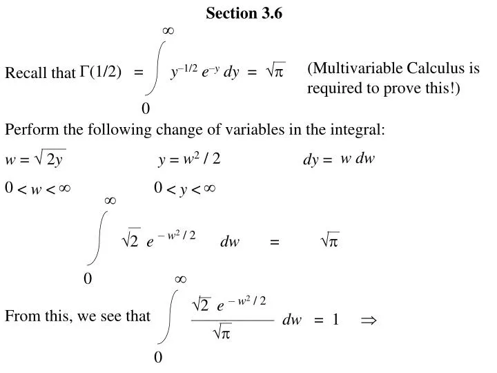
1. Section 3.6 Recall that  (Multivariable Calculus is required to prove this!) (1/2) = y–1/2e–y dy =  0 Perform the following change of variables in the integral: w =  2yy = dy = < w < < y < w dw w2 / 2 0  0   – w2 / 2 2 e dw =  0  – w2 / 2 2 e ————— dw = 1   From this, we see that 0

2.   – w2 / 2 – w2 / 2 2 e ————— dw = 2   e ——— dw = 1 2 –  –  Let –< a <  and 0 < b < , and perform the following change of variables in the integral: x = a + bww = dw = < x < < w < We shall come back to this derivation later. Right now skip to the following: A random variable having this p.d.f. is said to have a normal distribution with mean  and variance 2, that is, a N(,2) distribution. A random variable Z having a N(0,1) distribution, called a standard normal distribution, has p.d.f. – z2 / 2 e f(z) = ——— for –< z <  2

3. We let (z) = P(Z z), the distribution function of Z. Since f(z) is a symmetric function, it is easy to see that (– z) = 1 – (z). Tables Va and Vb in Appendix B of the text display a graph of f(z) and values of (z) and (– z). Important Theorems in the Text: If X is N(,2), then Z = (X– ) /  is N(0,1). Theorem 3.6-1 If X is N(,2), then V = [(X – ) / ]2 is 2(1). Theorem 3.6-2 We shall discuss these theorems later. Right now go to Class Exercise #1:

4. 1. The random variable Z is N(0, 1). Find each of the following: P(Z < 1.25) = (1.25) = 0.8944 P(Z > 0.75) = 1 – (0.75) = 0.2266 P(Z < – 1.25) = (– 1.25) = 1 – (1.25) = 0.1056 P(Z > – 0.75) = 1 – (– 0.75) = 1 – (1 – (0.75)) = (0.75) = 0.7734 P(– 1 < Z < 2) = (2)– (– 1) = (2)– (1 – (1)) = 0.8185 P(– 2 < Z < – 1) = (– 1)– (– 2) = (1 – (1))– (1 – (2)) = 0.1359 P(Z < 6) = (6) = practically 1

5. a constant c such that P(Z < c) = 0.591 P(Z < c) = 0.591 (c) = 0.591 c = 0.23 a constant c such that P(Z < c) = 0.123 P(Z < c) = 0.123 (c) = 0.123 1 – (– c) = 0.123 (– c) = 0.877 – c = 1.16 c = –1.16 a constant c such that P(Z > c) = 0.25 P(Z > c) = 0.25 1 – (c) = 0.25 c 0.67 a constant c such that P(Z > c) = 0.90 P(Z > c) = 0.90 1 – (c) = 0.90 (– c) = 0.90 – c = 1.28 c = –1.28

6. 1.-continued z0.10 P(Z > z) =   1 – (z) =  z0.10 = 1.282 z0.90 P(Z > z) =   1 – (z) = (–z) =   1 – (–z) = 1 –   P(Z > –z) = 1 –  z1– = –z z0.90 = – z0.10 = –1.282 a constant c such that P(|Z| < c) = 0.99 P(– c < Z < c) = 0.99 P(Z < c) – P(Z < – c) = 0.99 (c) –(– c) = 0.99 (c) –(1 – (c)) = 0.99 (c) = 0.995 c = z0.005 = 2.576

7.   – w2 / 2 – w2 / 2 2 e ————— dw = 2   e ——— dw = 1 2 –  –  Let –< a <  and 0 < b < , and perform the following change of variables in the integral: x = a + bww = dw = < x < < w < (x – a) / b (1/b) dx –   –    (x – a)2 – ——— 2b2 The function of x being integrated can be the p.d.f. for a random variable X which has all real numbers as its space. e ———— dx = 1 b2 – 

8. The moment generating function of X is M(t) = E(etX) =   (x – a)2 – ——— 2b2 (x – a)2 –2b2tx – —————— 2b2 etx e ———— dx = b2 e ———— dx = b2 –  –   Let us consider the exponent (x – a)2 –2b2tx – —————— 2b2 exp{ } —————————— dx b2 (x – a)2 –2b2tx – —————— . 2b2 –  (x – a)2 –2b2tx – —————— = 2b2 x2 – 2ax + a2 –2b2tx – ————————— = 2b2 x2 – 2(a + b2t)x + (a + b2t)2 – 2ab2t – b4t2 – ————————————————— = 2b2

9. [x–(a + b2t)]2 – 2ab2t – b4t2 – ———————————— . Therefore, M(t) = 2b2  (x – a)2 –2b2tx – —————— 2b2 exp{ } —————————— dx = b2 –   [x –(a+b2t)]2 – —————— 2b2 b2t2 exp{at + ——} 2 b2t2 at + —— 2 exp{ } —————————— dx = b2 e –  b2t2 at + —— 2 M(t) = e for –< t <  b2t2 at + —— 2 M(t) = (a + b2t) e b2t2 at + —— 2 b2t2 at + —— 2 M(t) = (a + b2t)2e + b2 e

10. E(X) = M(0) = a E(X2) = M(0) = a2 + b2 Var(X) = a2 + b2– a2= b2 Since X has mean  = and variance 2 = , we can write the p.d.f of X as a b2 (x –)2 – ——— 22 e f(x) = ———— for –< x <  2 A random variable having this p.d.f. is said to have a normal distribution with mean  and variance 2, that is, a N(,2) distribution. A random variable Z having a N(0,1) distribution, called a standard normal distribution, has p.d.f. – z2 / 2 e f(z) = ——— for –< z <  2

11. We let (z) = P(Z z), the distribution function of Z. Since f(z) is a symmetric function, it is easy to see that (– z) = 1 – (z). Tables Va and Vb in Appendix B of the text display a graph of f(z) and values of (z) and (– z). Important Theorems in the Text: If X is N(,2), then Z = (X– ) /  is N(0,1). Theorem 3.6-1 If X is N(,2), then V = [(X – ) / ]2 is 2(1). Theorem 3.6-2

12. 2. The random variable X is N(10, 9). Use Theorem 3.6-1 to find each of the following: 6 – 10 X– 10 12 – 10 P( ——— < ——— < ———— ) = 3 3 3 P(6 < X < 12) = P(– 1.33 < Z < 0.67) = (0.67)– (– 1.33) = (0.67)– (1 – (1.33)) = 0.7486 – (1 – 0.9082) = 0.6568 X– 10 25 – 10 P( ——— > ———— ) = 3 3 P(X > 25) = P(Z > 5) = 1 – (5) = practically 0

13. 2.-continued a constant c such that P(|X – 10| < c) = 0.95 X– 10 c P( ——— < — ) = 0.95 3 3 P(|X – 10| < c) = 0.95 P(|Z| < c/3) = 0.95 (c/3) –(– c/3) = 0.95 (c/3) –(1 – (c/3)) = 0.95 (c/3) = 0.975 c/3 = z0.025 = 1.960 c = 5.880

14. 3. The random variable X is N(–7, 100). Find each of the following: X+ 7 0 + 7 P( ——— > —— ) = 10 10 P(X > 0) = P(Z > 0.7) = 1 – (0.7) = 0.2420 a constant c such that P(X > c) = 0.98 X+ 7 c +7 P( —— > —— ) = 0.98 10 10 P(X > c) = 0.98 P(Z > (c+7) / 10) = 0.98 1 – ((c+7) /10) = 0.98 ((c+7) /10) = 0.02 (c+7) /10 = z0.98 = –z0.02 = – 2.054 c = – 27.54

15. 3.-continued X2+ 14X + 49 —————— 100 the distribution for the random variable Q = X2+ 14X + 49 —————— = 100 From Theorem 3.6-2, we know that Q = 2 X + 7 —— 10 must have a distribution. 2(1)