Download
1 / 61
640 likes | 1.02k Views
Theory of production. Production theory forms the foundation for the theory of supply Managerial decision making involves four types of production decisions: 1. Whether to produce or to shut down 2. How much output to produce 3. What input combination to use 4. What type of technology to use.

E N D
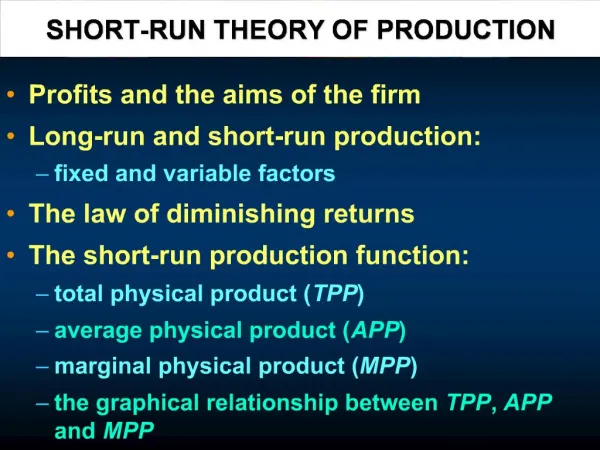
Production theory forms the foundation for the theory of supply • Managerial decision making involves four types of production decisions: 1. Whether to produce or to shut down 2. How much output to produce 3. What input combination to use 4. What type of technology to use
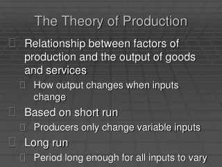
Production involves transformation of inputs such as capital, equipment, labor, and land into output - goods and services In this production process, the manager is concerned with efficiency in the use of the inputs - technical vs. economical efficiency
Two Concepts of Efficiency • Economic efficiency: • occurs when the cost of producing a given output is as low as possible • Technological efficiency: • occurs when it is not possible to increase output without increasing inputs
When a firm makes choices, it faces many constraints: • Constraints imposed by the firms customers • Constraints imposed by the firms competitors • Constraints imposed by nature Nature imposes constraints that there are only certain kinds of technological choices that are possible
The Technology of Production • The Production Process • Combining inputs or factors of production to achieve an output • Categories of Inputs (factors of production) • Labor • Materials • Capital
The Organization of Production • Inputs • Labor, Capital, Land • Fixed Inputs • Variable Inputs • Short Run • At least one input is fixed • Long Run • All inputs are variable
Long run and the short run • In the short run there are some factors of production that are fixed at pre-determined levels. (farming and land) • In the long run, all factors of production can be varied. • There is no specific time interval implied in the definition of short and long run. It depends on what kinds of choices we are examining
The Technology of Production • Production Function: • Indicates the highest output that a firm can produce for every specified combination of inputs given the state of technology. • Shows what is technically feasible when the firm operates efficiently.
TPL MPL = TP L APL = MPLAPL EL = Production Functionwith One Variable Input Total Product TP = Q = f(L) Marginal Product Average Product Production orOutput Elasticity
TCL Optimal Use of theVariable Input Marginal RevenueProduct of Labor MRPL = (MPL)(MR) Marginal ResourceCost of Labor MRCL = MRPL = MRCL Optimal Use of Labor
Production with TwoVariable Inputs Isoquants show combinations of two inputs that can produce the same level of output. Firms will only use combinations of two inputs that are in the economic region of production, which is defined by the portion of each isoquant that is negatively sloped.
A B C Q1 Q2 Q3 Isoquants When Inputs are Perfectly Substitutable Capital per month Labor per month
Production withTwo Variable Inputs Perfect Substitutes • Observations when inputs are perfectly substitutable: 1) The MRTS is constant at all points on the isoquant.
Production withTwo Variable Inputs Perfect Substitutes • Observations when inputs are perfectly substitutable: 2) For a given output, any combination of inputs can be chosen (A, B, or C) to generate the same level of output (e.g. toll booths & musical instruments)
Q3 C Q2 B Q1 K1 A L1 Fixed-ProportionsProduction Function Capital per month Labor per month
Production withTwo Variable Inputs Fixed-Proportions Production Function • Observations when inputs must be in a fixed-proportion: 1) No substitution is possible.Each output requires a specific amount of each input (e.g. labor and jackhammers).
Production withTwo Variable Inputs Fixed-Proportions Production Function • Observations when inputs must be in a fixed-proportion: 2) To increase output requires more labor and capital (i.e. moving from A to B to C which is technically efficient).
Production with TwoVariable Inputs Marginal Rate of Technical Substitution MRTS = -K/L = MPL/MPK
Curves showing all possible combinations of inputs that yield the same output An isoquant is a curve showing all possible combinations of inputs physically capable of producing a given fixed level of output The isoquants emphasize how different input combinations can be used to produce the same output. This information allows the producer to respond efficiently to changes in the markets for inputs.
Example 2 Production Table Units of K Employed Isoquant
Isocost Line • Isocost line: shows all possible K/L combos that can be purchased for a given TC. • TC = C = w*L + r*K ; • Rewrite as equation of a line: K = C/r – (w/r)*L Slope = K/L = -(w/r). • Interpret slope: * shows rate at which K and L can be traded off, keeping TC the same. • Relate to consumer’s budget constraint: * slope = ratio of prices with price from horizontal axis in numerator. Vertical intercept = C/r. Horizontal intercept = C/w.
Production and Costs Optimal combination of multiple inputs Shift Slope Isocost curves. All combinations of products that can be purchased for a fixed dollar amount Units of Y 12 10 Downward sloping curve. 8 B = $1,000 1 B = $2,000 2 6 B = $3,000 3 4 2 Units of X 0 2 4 6
Optimal Combination of Inputs Isocost lines represent all combinations of two inputs that a firm can purchase with the same total cost.
Production and Costs Optimal combination of multiple inputs Optimal combination corresponds to the point of tangency of the isoquant and isocost. Y Units of B 3 B 2 B 1 Expansion path Y 3 C Y 2 B Y 1 A Q 3 Q 2 Q 1 X X X 1 2 3 X Units of
Production and Costs Optimal combination of multiple inputs Optimal combination corresponds to the point of tangency isoquant and isocost. • Budget Lines • Least-cost production occurs when MPX/PX = MPY/PY and PX/PY = MPX/MPY • Expansion Path • Shows efficient input combinations as output grows. • Illustration of Optimal Input Proportions • Input proportions are optimal when no additional output could be produced for the same cost. • Optimal input proportions is a necessary but not sufficient condition for profit maximization. Units of Y B 3 B 2 B 1 Expansion path Y 3 C Y 2 B Y 1 A Q 3 Q 2 Q 1 X X X 1 2 3 Units of X
Production and Costs Optimal combination of multiple inputs Optimal combination corresponds to the point of tangency isoquant and isocost. • Profits are maximized when MRPX = PX for all inputs. • Profit maximization requires optimal input proportions plus an optimal level of output. Units of Y B 3 B 2 B 1 Expansion path Y 3 C Y 2 B Y 1 A Q 3 Q 2 Q 1 X X X 1 2 3 Units of X
Returns to Scale Production Function Q = f(L, K) Q = f(hL, hK) If = h, then f has constant returns to scale. If > h, then f has increasing returns to scale. If < h, then f has decreasing returns to scale.
Returns to Scale • Measuring the relationship between the scale (size) of a firm and output 1) Increasing returns to scale: output more than doubles when all inputs are doubled • Larger output associated with lower cost (autos) • One firm is more efficient than many (utilities) • The isoquants get closer together
Increasing Returns: The isoquants move closer together A 4 30 20 2 10 0 5 10 Returns to Scale Capital (machine hours) Labor (hours)
Returns to Scale • Measuring the relationship between the scale (size) of a firm and output 2) Constant returns to scale: output doubles when all inputs are doubled • Size does not affect productivity • May have a large number of producers • Isoquants are equidistant apart
A 6 30 4 20 2 10 0 5 10 15 Returns to Scale Capital (machine hours) Constant Returns: Isoquants are equally spaced Labor (hours)
Returns to Scale • Measuring the relationship between the scale (size) of a firm and output 3) Decreasing returns to scale: output less than doubles when all inputs are doubled • Decreasing efficiency with large size • Reduction of entrepreneurial abilities • Isoquants become farther apart