Download
1 / 76
780 likes | 1.08k Views
Crowd Simulation I. Introduction to Microscopic Crowd Simulation Techniques. Outline. Introduction to Crowd Simulation Fields of Study & Applications Visualization vs. Realism Microscopic vs. Macroscopic Flocking Social Forces 2D Cellular Automaton. Introduction.

E N D
Crowd Simulation I Introduction to Microscopic Crowd Simulation Techniques
Outline • Introduction to Crowd Simulation • Fields of Study & Applications • Visualization vs. Realism • Microscopic vs. Macroscopic • Flocking • Social Forces • 2D Cellular Automaton
Introduction • Crowd simulation attempts to model the motions of objects within an environment. • The topic has been researched from several different areas of study: • Entertainment and Visual Effects • Architecture and Civil Engineering • Psychology • Computer Science
Applications of Crowd Simulation • Entertainment and Visual Effects • Goal: Create a visually realistic model of crowds for use in movies, television, and video games. • Architecture and Civil Engineering • Goal: Study the flow of people/vehicles through environments. • Analyze road network efficiency. • Building evacuation characteristics. • Psychology • Goal: Validate behavior models of the human mind under different environmental conditions (ex. panic). • Computer Science • Goal: • Help out in any of the three areas above with algorithmic know-how. • Study AI models and behavior.
Visualization vs. Realism • The various crowd simulation techniques can generally be divided into two categories: • Visualization • Entertainment and Visual Effects • Realism • Architecture and Civil Engineering • Psychology • Techniques have begun to merge over the last decade.
Crowd Visualization • Goal: Create a visually realistic model of crowds. • Simulation does not have to be physically accurate. • Techniques may have to integrate with motion captured animations. • Algorithms frequently exploit Level-of-Detail. • Movies and television applications can afford offline processing as long as simulation time is reasonable. • Video games have real-time requirements.
Crowd Visualization Lord of the Rings Trilogy (2000 – 2003). Using the tool “Massive.” Disney’s Lion King (1994).
Crowd Realism • Goal: Study the flow of people/vehicles through environments. • Must be as physically accurate as possible. • Studies constantly compare simulation results with empirical data. • Simple visualizations such as a single point per object. • May have a very high order of objects to simulate.
Crowd Realism Simulation of a ship evacuation, using the tool EXODUS. Paths of pedestrian exploration driven by space syntax architectural concepts.
Microscopic vs. Macroscopic • Simulations techniques can also be categorized as microscopic vs. macroscopic. • Microscopic techniques simulate the individual object. • Crowd behavior is an emergent property of the microscopic-level algorithms driving the simulation. • Macroscopic techniques simulate groups of objects. • Example: Treating a transit system as a flow problem. • The rest of this lecture will study three different approaches to microscopic crowd simulation techniques.
Flocking • Flocking technique introduced by Craig W. Reynolds and his Boids. • Techniques to simulate animal flocking, herds, and schooling. • Sets the stage for further study into crowd simulation. • Each agent in the simulation is called a “boid.” • Big Idea: Complex crowd behaviors can be achieved through individual agents following simple rules.
Demos • Boids: • http://www.red3d.com/cwr/boids/applet/ • Disney’s Lion King: • http://www.youtube.com/watch?v=ruNv7uATZTQ • How was this done?
Flocking – Geometry in Flight • Each boid has its own local coordinate system: • X axis is left/right • Y axis is up/down • Z axis is ahead/back • Rotations too: • Rotation about X is pitch • Rotation about Y is yaw • Rotation about Z is roll • Each boid moves along its positive Z axis where pitch and yaw realign the global orientation of the Z axis.
Flocking – Geometry in Flight (3) • For realism in the simulation… • Momentum is conserved. • Speed dampening achieved by setting a maximum speed and acceleration. • Gravity is only used for banking of boids. • Banking orientation a function of path curvature and direction of gravity. • Not physically realistic. Does not capture that traveling up is harder than traveling down.
Flocking – Steering Behaviors • Flocking is closely related to particle systems. • Forces between particles cause motion. • Interactions take place within a local neighborhood of each Boid. • Three basic steering behaviors: • Separation • Alignment • Cohesion • Each steering behavior directs thrust in a desired direction.
Flocking – Steering Behaviors (2) • Separation • Boids steer to avoid crowding local flockmates. • Collision avoidance. • Keeps boids a realistic distance apart.
Flocking – Steering Behaviors (3) • Alignment (AKA Velocity Matching) • Boids attempt to match the velocity of their neighbors. • Complements separation. • Causes boids to move in the same general direction.
Flocking – Steering Behaviors (4) • Cohesion • Boids steer to move towards the average position of local flockmates. • Causes boids to keep together in a local flock. • Allows flocks to both merge and bifurcate.
Flocking – Boid Brain • Each steering behavior may yield a different thrust vector. • The Boid Brain combines, prioritizes, and arbitrates between potentially conflicting urges.
Flocking – Boid Brain (2) • Averaging (and weighted averaging) of steering vectors works “pretty well” but can yield poor behavior in cases where steering urges are in opposite directions. • Hesitation or indecision can lead to collisions with obstacles. • Example: • (Turn -90 degrees + Turn 90 degrees) / 2 = 0.
Flocking – Boid Brain (3) • Better Solution: • A fixed amount of “acceleration” is available to each boid each simulation iteration. • Steering vectors are processed in order of priority with a weighted average. • Priorities may be reassigned dynamically. • Steering vectors are processed until all acceleration credits have been used up. • The last processed vector is attenuated to keep within acceleration credit limits.
Flocking – Simulated Perception • As mentioned earlier, boid perception is limited to a local field of view. • Local neighborhood is a spherical zone of sensitivity centered around a boid’s origin. • Sensitivity is weighted with the inverse exponential of distance. (1/r2) • Early Boid implementation used linear weighting which yielded unrealistic spring-like animations. • Additional parameters can be used to simulated different fields of view: • Extra weighting in forward direction to increase awareness of what is ahead.
Flocking – Simulated Perception (2) • Implications of local perception: • Flocks of boids are allowed to bifurcate as groups of boids may break away from others and still satisfy the cohesion steering behavior. • Global cohesion/centering models were used early in Boids’ development. • Generated unusual effects causing all members of a scattered flock to simultaneously converge towards the flock’s centroid. • Spatially-oriented data structures may be used to reduce complexity below O(n2).
Social Forces • Developed by Dirk Helbing and Peter Molnar in 1995 with several advancements over the last decade. • Later contributions from Illes Farkas and Tamas Vicsek. • A frequently referenced piece of work. • Widely successful because it elegantly reproduces many common features observed in pedestrian movement.
Social Forces • Social Forces are not exerted by the environment on a pedestrian’s body, but rather a quantity that describes the motivation to act. • Respect personal space. • Follow others at a safe distance. • Avoid getting too close to walls and obstacles. • Can be thought of as a developed model of “flocking for human pedestrians” as humans follow a set of social rules that guide their movement.
Social Forces ’95 – Equations • Desired Motion • Obstacle Avoidance • Social Force • Attractive Forces • Let’s work backwards. Here’s the equation describing all forces acting on an individual agent:
Social Forces ’95 – Equations • Acceleration towards a goal. • Given current location, desired location, current speed, and desired speed, an equation describing acceleration towards the destination is given by: • Where eα is a unit vector towards the destination. • The ταterm is a relaxation time that causes a delay after the agent has performed deceleration processes.
Social Forces ’95 – Equations • Respect the personal space of others. • Pedestrians will keep a certain distance from others that depends upon the pedestrian density and desired speed. • This behavior can be implemented as a repulsive force between agents with the following equations: • Where Vαβ is a monotonic decreasing function of b with equipotential lines having the form of an ellipse that is in the direction of motion. • Elliptical range allows for an agent to leave room for their own subsequent steps. • Helbinget al later revise and simplify this equation in 2000. This will be discussed in a little bit.
Social Forces ’95 – Equations • Respect the personal space of others. (cont.) • Pedestrians have a limited cone of vision, so forces from agents outside an agent’s immediate attention should be attenuated. • This is done with the following weight function: • This gives us the final inter-agent repulsive forces: • Care must be taken for inter-agent forces to not cross between obstacles. For example, agents on opposite sides of a wall should not affect each other.
Social Forces ’95 – Equations • Avoid colliding with obstacles. • Pedestrians will also keep a certain distance from borders of buildings, walls, obstacles, etc. to avoid injury. • This behavior can be described by the following: • Where UαB is a monotonic decreasing potential. • The vector rαB denotes the distance between the agent and the nearest portion of the obstacle.
Social Forces ’95 – Equations • Social Forces also allows attractive forces. • Examples: • Friends • Street Performers • Window Displays • The equation for these forces has the same form as the inter-agent repulsive forces. • This force is also attenuated with a field of attention, giving:
Social Forces ’95 – Equations • Here is the final Social Force equation one more time: • The social force model is now defined by: • The fluctuation term takes into account random variations in behavior. Enhances realism. m/s2
Social Forces ’95 – Equations • The previous equation described changes in acceleration. • Changes in velocity are given by the following equation: • The trailing g-term caps speed. m/s
Social Forces ’95 – Simulations • Repulsive potentials were assumed decrease exponentially: • Parameter values: • Voαβ = 2.1m2/s2 • σ= 0.3m • UoαB = 10m2/s2 • R = 0.2m • τα = 0.5s (smaller times more aggressive)
Social Forces ’95 – Simulations (2) • Two pedestrian phenomena were observed with these equations: • Lane Formation • Door Oscillation
Social Forces ’95 – Simulations (3) • Lane Formation • The empty circles and full circles have desired direction of motion in opposite directions. • Circle diameter reflects actual velocity.
Social Forces ’95 – Simulations (4) • Door Oscillation • If one pedestrian has been able to pass a narrow door, other pedestrians with the same desired walking direction can follow easily. Others have to wait. • The door can be “captured” as pressure on the opposite side builds up, allowing pedestrians in the other direction to pass.
Social Forces – Additions • Several additions to Social Forces has been made over the years. • In 2000, the equations were revised to study panic and evacuation dynamics. • Characteristics of panic: • People move or try to move considerably faster than normal. • Individuals start pushing each other (violating repulsive forces from earlier work). • Moving becomes uncoordinated. • Arching and clogging appears at exits. • Jams build up. • Physical interactions in jams can build up to dangerous pressures, injuring people and breaking of obstacles. • Injured people become obstacles to the rest of the crowd. • People show a tendency towards mass behavior. • Alternative exits are often overlooked or not efficiently used. • The bold items were addressed in 2000.
Social Forces ’00 – Equations • The revised inter-agent force equation is given by: • “Body force” counteracts body compression. k is a large constant. • “Sliding friction force” impedes relative tangential motion if pedestrians come too close. Κ is another large constant. • Inspired by granular interactions. • Obstacle repulsion force updated in the same manner.
Social Forces ’00 – Equations • The desired direction of motion updated to also include mass behavior: • Simulations found that a mix of both individual and mass directions worked best. • Panic (high mass behavior) is realized through a high pi value.
Social Forces ’00 – Simulations • Arching/Clogging at exits:
Social Forces ’00 – Simulations • Corridor widening can lead to bottlenecks:
Social Forces ’00 – Simulations • Mass behavior and inefficient use of exits:
Social Forces – More Results • Below shows the effects of fire, which is said to have a socio-psychological strength 10x greater than a normal wall. • Incapacitated agents are shown as full circles.
Social Forces – More Results (2) • Suggestions for improved motion. • Environments more conducive to efficient motion are shown on the right.
Social Forces – More Results (3) • Breaking of a corridor doorway into two helps in lane formation and avoid door clogging and oscillation.
Social Forces – More Results (4) • Placing a column in front of an exit can alleviates problems due to arching by reducing pressure. • More efficient egress. • Fewer or no injuries. • Injured agents are shown as full circles on the left.