Download
1 / 16
170 likes | 373 Views
20. y = 0.54x - 1.2. 2. R. = 0.56. 15. Species of local pool. 10. 5. 0. 0. 10. 20. 30. Species of regional pool. Local and regional species richness . Bracken occurs whole over the world Species numbers of phytophages on bracken differ

E N D
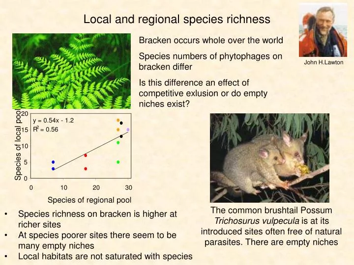
20 y = 0.54x - 1.2 2 R = 0.56 15 Species of local pool 10 5 0 0 10 20 30 Species of regional pool Local and regional species richness Brackenoccurswholeovertheworld Speciesnumbers of phytophages on brackendiffer Isthisdifference an effect of competitiveexlusionor do emptynichesexist? John H.Lawton ThecommonbrushtailPossumTrichosurusvulpeculaisatitsintroducedsitesoftenfree of natural parasites. Thereareemptyniches • Speciesrichness on brackenishigheratrichersites • Atspeciespoorersitesthereseem to be many emptyniches • Localhabitatsare not saturatedwithspecies
25 4 y = 0.36x + 0.41 y = 0.49x + 0.51 3.5 20 2 R = 0.83 2 R = 0.73 3 2.5 15 Number of species locally Local number of species 2 10 1.5 1 5 0.5 0 0 0 10 20 30 40 0 2 4 6 8 10 Number of species regionally Regional number of species 120 120 y = 0.27x - 6.9 y = 16Ln(x) - 49 100 100 R 2 = 0.93 R 2 = 0.86 80 80 Number of species locally Number of species locally 60 60 40 40 20 20 0 0 0 100 200 300 400 0 100 200 300 400 Number of species regionally Number of species regionally Local and regionalspeciesrichness Lacutrine fish in North America (Gaston 2000) Cynipid gall wasps in Norh America (Cornell 1985) Relationship between local species richness and the regional species pool sizefor 14 vegetation types in Estonia (Pärtel et al. 1996) Drygrasslands Moist grasslands
40 35 30 25 Local number of species 20 15 10 5 0 0 10 20 30 40 Regional number of species Four possible relations between local and regional species numbers
30% 8 6.97x 2.58x y = 0.067e y = 0.95e 25% 6 2 2 R = 0.5472 R = 0.83 20% Mean abundance Percentage of total Abundance 15% 4 10% 2 5% 0 0% 0 0.2 0.4 0.6 0.8 0 0.05 0.1 0.15 0.2 Fraction of pools occupied Fraction of sites occupied 1000 80 0.11x y = 3.06e 0.33x y = 1.0e 800 2 60 R = 0.90 2 R = 0.82 600 log rel. abundance log rel. abundance 40 400 20 200 0 0 0 10 20 30 40 50 0 2 4 6 8 10 Number of sites occupied Number of sites occupied 80 10 3.674x 2.97x y = 1.35e y = 1.57e 8 60 2 2 R = 0.59 R = 0.78 6 Mean density per Mean density per occupied patch occupied patch 40 4 20 2 0 0 0% 20% 40% 60% 80% 100% 0% 20% 40% 60% Percentage of site occupied Percentage of site occupied Abundance – rangesizerelationships Freshwatergyrinid beetles in temporary pools (Svensson 1992) Regional distribution of 21 Bombus species in northern Spain (Obeso 1992) Local abundance in relation to regional distribution of soil mites (Karppinen 1958) D: Local abundance in relation to regional distribution of bumblebees in Poland (Anasiewicz 1971) Parasitic Hymenoptera of these Diptera (Ulrich 2001) Diptera colonising dead snails in a beech forest (Ulrich 2001)
40 1.61x y = 6e 30 2 R = 0.60 Mean density per 20 occupied cell 10 0 0.01 0.1 1 Fraction of cells occupied Patch occupancy models 4 4 2 5 4 4 4 20 1 3 3 5 1 8 1 17 12 Individuals of 100 specieswereplacedat random into a 100x100 matrix. Specieshaddifferentindividualnumbers Matrixcellshaddifferentcapacities • A matrix of cellsrefers to a metacommunityscale • Eachcellrepresents one local community • Cellsmighthavedifferentsizes • Individuals of differentspecies of themeta-community arenowplacedat random oraccording to certainpredefinedrulesintothecells • A random placementiscalled a passivesampling model • Thespatialdistributionpatternsarethencompared to observedones. • The model produces an abundance - rangesizerelationship • Thisrelationshipfollows an exponential model as observedin reality • Abundance - rangesizerelationshipsare most parsimonousexplainedfrompassivesamplinginheterogeneousenvironments
80 100 80 60 60 Number of species Number of species 40 40 20 20 0 0 1 2 3 4 5 6 7 8 9 0 1 2 3 4 5 6 7 8 9 10 11 12 Number of sites occupied Number of sites occupied Core and satellite species Plant species in Russian Karelia (Linkola 1916) Insects on small mangrove islands (Simberloff 1976) In an assemblage of species distributed over many sites we can often differentiate a group of core species, which occur in most or even all of the sites, and a group of satellite species, which occur only in a few or even only in one site.
Core and satellitespecies Groundbeetlesspecies on Mazuranlakeisland Core (frequent, permanent) species Satellite (infrequent, tourist) species • Random pattern of temporalorspatialoccurrence • High dispersalability • Log-seriesrankabundancedistributions • Weakspeciesinteractions • Forming random assemblages • Non-random pattern of temporalorspatialoccurrence • Lower dispersalability • Log-normalrankabundancedistributions • Importance of speciesinteractions • Forming trueecologicalcommunities Importance of ecologicalinteractions
Nestedness Groundbeetlesspecieswith limited dispersalability on Mazuranlakeisland Core and satellitespecies
Thematrixsortedaccording to row and columntotals (numbers of occurrences) containestwotriangles. One containspecies and sitewithvery high matrixfill (numbers of occurrences, thesecondcontainsspecies and sitewithverylowmatrixfill. We callsuch a matrixnested.
A perfectlynestedmatrix Imperfectlynestedmatriceshaveholes (unexpectedabsences) and outliers (unexpectedoccurrences). A perfectlynested (ordered) matrixcan be dividedinto a completelyfilled and an empty part. Thenumber of holes and outlierwithrespect to theperfectlyordered state is a measure of thedegree of nestedness. Thediscrepancymetriccountsthenumber of holesthathave to be filled by outliers of the same roworcolumn to form a perfectlynestedmatrix.
Nestedness analysissurves to findidiosyncraticspeciesthatmeansspeciesthatdeviatefromthe general trend of community organization. .Oftenthesespecies do not belong to theguild of species under studywhilehavingdifferent habitat requirements.
Analysis of ecologicalgradients Nestedness analysisisparticulalry an analysis of ecologicalgradients Nestedness analysishelps to identifyspeciesthat run counter to ecologicalgradients
Statisticalinferenceusingnullmodels Checkerboards We randomizethematrixswitchingcheckerboards. Thisretainsrow and columntotals and thereforebasicmatrixproperties. Observeddiscrepancy D = 11 We have to inferhow many discrepanciesareexpectedjust by chance. 1. Use 10*sites*species checkerboardswaps per matrix to randomize. 2. Calculatediscrepancy. 3. Repeatsteps 1 and 2 1000 times to getthenulldistribtuion. 4. Comparetheobserveddiscepancywiththeexpected one. Antinested Nested Observed Upper 5% CL Lower 5% CL
Both matrices are not significantly nested. There are not more idiosyncratic sites and species than expected just by chance. Low dispersal Carabidae do not colonize lake island according to organic matter content (soil fertility). Our first eysight impression was wrong. Alwaysaskwhether an observedpatternorprocessmightexistjust by chance.
Today’s reading Local and regional species richness: http://www.springerlink.com/content/ugm5380764049730/ Nestedness and null models: www.uvm.edu/~ngotelli/manuscriptpdfs/UlrichConsumersGuide.pdf Community assembly: www.msstate.edu/courses/etl5/Community%20Assembly1.ppt