Download
1 / 1
10 likes | 162 Views
Ω. What is the induced radial electric field e?. Applied external magnetic field B 0. Albert Einstein. Michael Faraday. Ω. Rotating dielectric cylinder. What magnetic field is induced inside and outside the dielectric?. What’s the big argument about?. Yes – the Wilsons were right!.

E N D
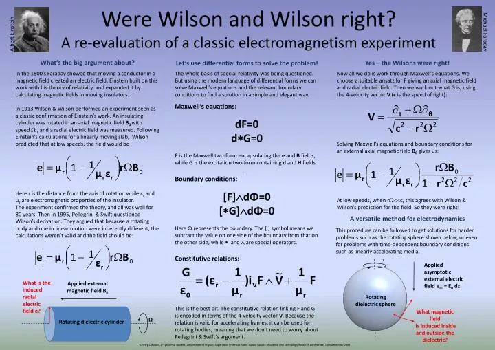
Ω What is the induced radial electric field e? Applied external magnetic field B0 Albert Einstein Michael Faraday Ω Rotating dielectric cylinder What magnetic field is induced inside and outside the dielectric? What’s the big argument about? Yes – the Wilsons were right! Let’s use differential forms to solve the problem! In the 1800’s Faraday showed that moving a conductor in a magnetic field created an electric field. Einstein built on this work with his theory of relativity, and expanded it by calculating magnetic fields in moving insulators. In 1913 Wilson & Wilson performed an experiment seen as a classic confirmation of Einstein’s work. An insulating cylinder was rotated in an axial magnetic field B0 with speed , and a radial electric field was measured. Following Einstein’s calculations for a linearly moving slab, Wilson predicted that at low speeds, the field would be Here r is the distance from the axis of rotation while r and r are electromagnetic properties of the insulator. The experiment confirmed the theory, and all was well for 80 years. Then in 1995, Pellegrini & Swift questioned Wilson’s derivation. They argued that because a rotating body and one in linear motion were inherently different, the calculations weren’t valid and the field should be: The whole basis of special relativity was being questioned. But using the modern language of differential forms we can solve Maxwell’s equations and the relevant boundary conditions to find a solution in a simple and elegant way. Now all we do is work through Maxwell’s equations. We choose a suitable ansatz for F giving an axial magnetic field and radial electric field. Then we work out what G is, using the 4-velocity vector V (c is the speed of light): Solving Maxwell’s equations and boundary conditions for an external axial magnetic field B0gives us: At low speeds, when rc, this agrees with Wilson & Wilson’s prediction for the field. So they were right! Maxwell’s equations: dF=0 dG=0 F is the Maxwell two-form encapsulating the e and B fields, while G is the excitation two-form containing d and H fields. Boundary conditions: [F]dΦ=0 [G]dΦ=0 Here Φ represents the boundary. The [ ] symbol means we subtract the value on one side of the boundary from that on the other side, while and are special operators. Constitutive relations: This is the best bit. The constitutive relation linking F and G is encoded in terms of the 4-velocity vector V. Because the relation is valid for accelerating frames, it can be used for rotating bodies, meaning that we don’t need to worry about Pellegrini & Swift’s argument. Were Wilson and Wilson right?A re-evaluation of a classic electromagnetism experiment Rotating dielectric sphere A versatile method for electrodynamics This procedure can be followed to get solutions for harder problems such as the rotating sphere shown below, or even for problems with time-dependent boundary conditions such as linearly accelerating media. Applied asymptotic external electric field e∞ = E0 dz Cherry Canovan, 2nd year PhD student, Department of Physics. Supervisor: Professor Robin Tucker. Faculty of Science and Technology Research Conference, 15th December 2009