The Multiplier Model

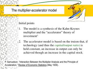
1. The Multiplier Model Chapter 10

2. LAUGHER CURVE �If you put two economists in a room, you get two opinions, unless one of them is Lord Keynes, in which case you get three opinions.� Winston Churchill

3. The Multiplier Model The last chapter covered how an initial shift in aggregate expenditure might shift the AD curve by a multiple amount but it was not stated by how much. The multiplier model tells us how much AD may shift.

4. The Multiplier Model The multiplier model assumes that the price level remains constant - and then explores specific questions about expenditures.

5. The Multiplier Model The multiplier model gives numerical answers about the effect of changes in aggregate expenditures on aggregate output.

6. The AS/AD Model When Prices Are Fixed

7. Aggregate Production Aggregate production (AP) is the total amount of goods and services produced in every industry in an economy.

8. Aggregate Production Production creates an equal amount of income.

9. Aggregate Production Graphically, aggregate production in the multiplier model is represented by a 45� line through the origin

10. Aggregate Production Real production (in dollars) is on the vertical axis, and real income (in dollars) is on the horizontal axis.

11. The Aggregate Production Curve

12. Aggregate Expenditures Aggregate expenditures (AE) in the multiplier model consist of: Consumption � spending by consumers. Investment � spending by business. Spending by government. Net foreign spending on U.S. goods � the difference between U.S. exports and U.S. imports.

13. Aggregate Expenditures The four expenditure components of national income accounting were developed contemporaneously with the multiplier model.

14. Autonomous and Induced Expenditures As income changes, expenditures change, but not as much as income.

15. Autonomous and Induced Expenditures Even if income is zero, spending is still taking place. The money comes from borrowing, or from previous savings.

16. Autonomous and Induced Expenditures Autonomous expenditures are those that would exist at a zero level of income. Autonomous expenditures are independent of income.

17. Autonomous and Induced Expenditures Autonomous expenditures change because something other than income changes.

18. Autonomous and Induced Expenditures Induced expenditures are those that change as income changes.

19. Aggregate Expenditures Related to Income

20. Expenditures Function The relationship between expenditures and income can be expressed more concisely as an expenditures function. An expenditures function is a representation of the relationship between expenditures and income.

21. Expenditures Function AE = expenditures AEo = autonomous expenditures mpc = marginal propensity to consume Y = income

22. The Marginal Propensity to Consume The marginal propensity to consume (mpc) is the ratio of a change in consumption (?C) to a change in income (??Y).

23. The Marginal Propensity to Consume The mpc is the fraction spent from an additional dollar of income.

24. The Marginal Propensity to Consume The mpc captures the rule of thumb that individuals in aggregate tend to follow:

25. The Marginal Propensity to Consume Since only consumption expenditures depend on income, in our simple model:

26. Graphing the Expenditures Function The graphical representation of the expenditures function is called the aggregate expenditures curve. The expenditures function's slope tells us how much expenditures change with a particular change in income.

27. Graphing the Expenditures Function It is assumed that only consumption changes with income; the other expenditure components � I, G, (X - M) � are all independent of income.

28. Graphing the Expenditures Function

29. Shifts in the Expenditures Function The expenditure function shifts up and down when autonomous C, I, G, or X - M change. The reason that these shifts are so important is that the multiplier model is an historical model in time.

30. Shifts in the Expenditures Function The multiplier model can be used to analyze shifts in aggregate expenditures from an historically given level.

31. Determining the Level of Aggregate Income In bringing AP and AE together in one framework, the following is assumed : The price level is constant. The AP curve is a 45o line until the economy reaches its potential income. Expenditures shown on the AE line do not necessarily equal AP or income.

32. Determining the Level of Aggregate Income To determine income graphically, you find the income level at which AE equals AP.

33. Solving for Equilibrium Graphically

34. The Multiplier Equation The multiplier equation tells us that income equals the multiplier times autonomous expenditures. Y = (multiplier)(autonomous expenditures)

35. The Multiplier Equation The multiplier equation is a useful way to determine the level of income in the multiplier model.

36. The Multiplier Equation The multiplier is a number that reveals how much income will change in response to a change in autonomous expenditures.

37. The Multiplier Equation As the mpc increases, the multiplier increases:

38. The Multiplier Process The multiplier process amplifies changes in autonomous expenditures. What forces are operating to ensure that the income level we determined is actually the equilibrium income level?

39. The Multiplier Process When expenditures do not equal current output, business people change planned production:

40. The Multiplier Process

41. The Circular Flow Model and the Multiplier Process The circular flow model provides the intuition behind the multiplier process.

42. The Circular Flow Model and the Multiplier Process Expenditures are injections into the circular flow.

43. The Circular Flow Model and the Multiplier Process Economists use the term the marginal propensity of save (mps) to represent the percentage of income flow that leaks out of the economy for each round of the circular flow.

44. The Circular Flow Model and the Multiplier Process By definition:

45. The Circular Flow Model and the Multiplier Process

46. The Multiplier Model in Action The first step in understanding the AP/AE analysis is determining the level of income using the multiplier. This was already explained.

47. The Multiplier Model in Action The second step is to modify that analysis to answer a question that is of much more interest to policy makers.

48. The Multiplier Model in Action Autonomous expenditures are determined outside the model not as a result of changes in income.

49. The Steps of the Multiplier Process The income adjustment process is directly related to the multiplier. Any initial shock (a change in autonomous AE) is multiplied in the adjustment process.

50. The Steps of the Multiplier Process The multiplier process repeats and repeats until a new equilibrium level is finally reached.

51. Shifts in the Aggregate Expenditure Curve

52. The First Five Steps of Four Multipliers

53. The First Five Steps of Four Multipliers

54. The Effect of Shifts in Aggregate Expenditures Autonomous expenditures can, and do, shift for a number of reasons: Natural disasters. Sudden climatic changes. Changes in consumption causes by changes in consumer choice.

55. The Effect of Shifts in Aggregate Expenditures Autonomous expenditures can, and do, shift for a number of reasons:

56. The Effect of Shifts in Aggregate Expenditures An understanding of these shifts can be enhanced by tying them to the formula: AE = C + I + G + (X - M)

57. The Effect of Shifts in Aggregate Expenditures An understanding of these shifts can be enhanced by tying them to the formula: AE = C + I + G + (X - M)

58. The Effect of Shifts in Aggregate Expenditures Changes in consumer sentiment affect C.

59. The Effect of Shifts in Aggregate Expenditures

60. Shifts in Autonomous Expenditures

61. Shifts in Autonomous Expenditures

62. Shifts in Autonomous Expenditures

63. An Upward Shift of AE

64. An Downward Shift of AE

65. Real World Examples The United States in 1998. Japan in the 1990s. The 1930s depression.

66. The United States in 1998 Consumer confidence rose substantially causing autonomous consumption expenditures to increase more than economists had predicted. While economists had expected the economy to grow slowly, it boomed.

67. Japan in the 1990s A dramatic rise in the yen cut Japanese exports. Suppliers could not sell all they had produced.

68. Japan in the 1990s Suppliers laid off workers and decreased output.

69. The 1930s Depression The 1929 stock market crash, which continued into 1930, threw the financial markets into chaos. This resulted in a downward shift of the AE curve.

70. The 1930s Depression Frightened business people decreased investment and laid off workers.

71. The 1930s Depression Business people responded by decreasing output, which decreased income, starting a downward cycle, thereby confirming the fears of the businesspeople.

72. The 1930s Depression The process continued until the economy settled at a low-level equilibrium, far below the potential level of income.

73. The 1930s Depression The process caused the paradox of thrift, whereby individuals attempting to save more, spent less, and caused income to decrease.

74. Limitations of the Multiplier Model On the surface, the multiplier model makes a lot of intuitive sense. Surface sense can often be misleading.

75. The Multiplier Model Is Not a Complete Model The multiplier model does not determine income from scratch. At best, it can estimate the directions and rough sizes of autonomous demand or supply shifts.

76. Shifts Are Not as Great as Intuition Suggests The multiplier model leads people to overemphasize the aggregate expenditure shifts that would occur in response to a shift in autonomous expenditures.

77. The Price Level Will Often Change in Response to Shifts in Demand The multiplier model assumes that the price level is fixed. The price level can change in response to changes in aggregate demand. Price level changes will occur when the economy is in the intermediate range.

78. Forward-Looking Expectations Complicate the Adjustment Process People's forward-looking expectations make the adjustment process much more complicated. Most people, however, act upon their expectations of the future.

79. Forward-Looking Expectations Complicate the Adjustment Process Business people may not automatically cut back production and lay-off workers if they think a fall in sales is temporary.

80. Forward-Looking Expectations Complicate the Adjustment Process Some modern economists have put forward a rational expectations model of the economy.

81. Shifts in Expenditures Might Reflect Desired Shifts in Supply and Demand Shifts in demand can occur for many reasons. Many shifts can reflect desired shifts in aggregate production which are accompanied by shifts in aggregate demand.

82. Shifts in Expenditures Might Reflect Desired Shifts in Supply and Demand Shifts may be simultaneous shifts in supply and demand that do not necessarily reflect suppliers' responding to changes in demand.

83. Shifts in Expenditures Might Reflect Desired Shifts in Supply and Demand Expansion of this line of thought has led to the real business cycle theory of the economy.

84. Shifts in Expenditures Might Reflect Desired Shifts in Supply and Demand Real business cycle theory of the economy � fluctuations in the economy reflect real phenomena such as simultaneous shifts in supply and demand, not simply supply responses to demand shifts.

85. Expenditures Depend on Much More Than Current Income If people base their spending on lifetime income, not yearly income, the mpc out of changes in current income could be very low, even approaching zero.

86. Expenditures Depend on Much More Than Current Income In that case, the expenditures function would essentially by a flat line, and the multiplier would be one, and there would be no secondary effects of an initial shift.

87. Expenditures Depend on Much More Than Current Income This set of arguments is called the permanent income hypothesis.

88. The Multiplier Model End of Chapter 10