Download
1 / 37
460 likes | 1.06k Views
Using ANSYS. First load up ANSYS. Follow instructions given in the word document Iceberg_MPY308.doc Lets run in a directory called TEST1 So first issue the commands: mkdir TEST1 cd TEST1 If you now list your directory contents it should be empty: ls –l

E N D
First load up ANSYS • Follow instructions given in the word document Iceberg_MPY308.doc • Lets run in a directory called TEST1 • So first issue the commands: mkdir TEST1 cd TEST1 • If you now list your directory contents it should be empty: ls –l (this should give: total 0)
First load up ANSYS • Run ANSYS using: ansys –g & • You should get the graphical display • If you go back to your command window and list the directory contents, you should get (something similar to): total 8 -rw-r--r-- 1 mpp97ajn mp 0 Oct 26 17:40 file.err -rw-r--r-- 1 mpp97ajn mp 0 Oct 26 17:40 file.lock -rw-r--r-- 1 mpp97ajn mp 233 Oct 26 17:40 file.log -rw-r--r-- 1 mpp97ajn mp 0 Oct 26 17:40 file.page -rw-r--r-- 1 mpp97ajn mp 72 Oct 26 17:40 menust.tmp • These new files are created by ANSYS • The file.log file can be useful as it contains any commands you enter into ANSYS
Ways to use ANSYS You can do things graphically using the menus at the top and the side of the screen This will often bring up a dialog box or ask you to pick things with the cursor NOTE: You can change font size using the MenuCtrls > Font Selection menu
Graphical input • Try it! From the side menu select: Preprocessor > Modeling > Create > Areas > Rectangle > By 2 corners • This should bring up this dialog box • WP X and WP Y are the coords of the bottom left corner of the rectangle • Type a value for these and the width and height and click OK • You should get a cyan rectangle
ANSYS commands • Now look at your log file • Type nedit file.log & • This will open the file.log in a text editor, scroll down to the bottom and you will see: BLC4, val1 , val2 , val3 , val4 • This is the command to create a rectangle (val1 – val4 have been specified by you)
Using ANSYS commands • If you type a command in the command box, ANSYS will tell you what it expects as input data • Typing the command in has the same effect as running it graphically and the command will also be stored in the log file as before • To get help, simply type help in the command box, or use the help menu to select Help Topics
Input files • You can programme in ANSYS using input files • These are just text files containing a list of ANSYS commands: • Purple text is comment (designated by ‘!’) for info only !plate: ANSYS input file for plate with hole /FILNAM,plate! Name the file /PREP7! Enter the preprocessor ET,1,PLANE42! Define the element type - 4 node solid element UIMP,1,EX, , ,200000,! Define material properties K,1,2.5,0,,! Define keypoints LARC,1,2,11,2.5,! Define arcs LSTR, 1, 4! Define straight lines AL,3,6,4,1! Define areas lesize,3,,,15! Define mesh size
The database • You can save ANSYS models as a database file This can be done here or with the SAVE command • Once you have done this if you list the directory contents it now contains a file: file.db • You can resume from your database each time you start ANSYS File > Resume from OR RESUME
Why use input files? • They are small, large models can be built with only a few commands • They allow you to review what you’ve done easily • They allow you to modify models very quickly I have built and meshed a square in ANSYS, now I want to change the length of the model Graphically With an input file Either: Modify keypoints and then remesh the areas of the model Or: Start again from scratch File > Clear and start new Change 2 values in input file and run again: BLC4, val1 , val2 , val3 , val4 File > Read input from
Why use input files? • Parameterisation can be very useful /PREP7 ET,1,42 !Define the parameters of my problem xlength = 10 ylength = 20 xmesh = 5 ymesh = 15 !Use the parameters to define geometry and mesh the model BLC4, -xlength/2 , -ylength/2 , xlength , ylength LSEL,s,loc,x,0 LESIZE,all,,,xmesh LSEL,s,loc,y,0 LESIZE,all,,,ymesh AMESH,all We can define the mesh and geometry using just these 4 values
Geometry definition • Start by defining keypoints • Join keypoints together using lines • Mesh lines with 1d elements or…… • Create areas from lines • Mesh areas with 2d elements or….. • Create volumes from areas • Mesh volumes with 3d elements • In some cases it is quicker to use pre-defined geometry (like the rectangle command) which will automatically create kypts and lines
A note on units • ANSYS knows nothing about the units you are using • It is important to be consistent • For this example we will choose mm as our unit of length and MPa for stress • The consistent units of mass, time and force are then grams, ms and N respectively
6 5 8 3 2 11 1 4 7 Structural (1) • File > Clear and start new • File > Read input from (select file ANSYS_plate.in) • What does this do? Line by line: !plate: ANSYS input file for plate with hole /FILNAM,plate ! Sets the filename – all output files will be named plate from now on /PREP7! Enter the preprocessor – all geometry creation is done here ET,1,PLANE42! Define the element type - 4 node solid element, type help 42 for more info UIMP,1,EX, , ,200000,! Define material properties, this is the Young’s modulus in the x direction UIMP,1,NUXY, , ,0.3, ! Define material properties, this is the value of Poisson’s ratio for the material K,1,2.5,0,,! Define keypoints, format is: k,knum,kx,ky knum is the number of the point K,2,1.768,1.768,, ! knum is the number of the point, kx is the x coordinate, ky is the y coordinate K,3,0,2.5,, K,4,10,0,, K,5,10,10,, K,6,0,10,, K,7,50,0,, K,8,50,10,, K,11,0,0,, KEYPOINT LOCATIONS
8(8) 10(12) 6(8) 5(15) 7(8) 4(15) 2(8) 1(8) 3(15) 9(12) Structural (2) LARC,1,2,11,2.5, ! Define arcs LARC,2,3,11,2.5, ! format is: larc, pt1,pt2,cntr,radius LSTR, 1, 4 ! Define straight lines between kypts LSTR, 2, 5 LSTR, 3, 6 LSTR, 4, 5 LSTR, 7, 8 LSTR, 5, 6 LSTR, 4, 7 LSTR, 5, 8 AL,3,6,4,1 ! Define areas using line numbers AL,4,8,5,2 AL,9,7,10,6 lesize,3,,,15 ! Define mesh size lesize,4,,,15 ! The number of elements lesize,5,,,15 ! is specified per line lesize,1,,,8 lesize,2,,,8 lesize,6,,,8 lesize,7,,,8 lesize,8,,,8 lesize,9,,,12 lesize,10,,,12 amesh,1,3,1 !Mesh Areas ! Then define boundary conditions, loads ! Solve the model and post-process LINE NUMBERS AND (MESH SIZING) For ‘mapped meshing’ we need consistent sizing in the direction of the arrows – this can reduce the number of elements and generally creates a better mesh AREA NUMBERS and FINAL MESH GEOMETRY
Lines and kypts before NUMMRG 8 7 4 3 3 7 4 2 8 6 1 5 5 6 1 2 Lines and kypts after NUMMRG 3 7 4 3 3 7 4 2 2 6 1 2 5 6 1 2 Warning! Definition of model geometry • If you define areas and lines using BLC4 and other commands like it, they will not share boundaries • You can use NUMMRG,all,tol to merge common boundaries (tol is the tolerance, usually use very small value)
Structural (3) • What are the boundary conditions? • What are the degrees of freedom? • Help on element 42 tells us it has four nodes, with 2 DOF at each node, UX and UY • We are exploiting symmetry - so in the structural case we constrain displacements normal to the axis of symmetry • So we need to set UX = 0 on y axis (x=0) • So we need to set UY = 0 on x axis (y=0)
Structural (4) • How do we apply these conditions? Preprocessor > Loads > Define Loads > Apply > Structural > Displacement > Choose and then pick the nodes (or lines) you want using the cursor Select nodes by location using NSEL,s,loc,x,min,max where x,y or z is coordinate direction, min is the minimum value in this direction, max is the maximum value (if only one value is given, just the nodes at this exact location are selected). Apply DOF constraints to selected nodes using D,nnum,DOF,val where nnum is the number of the node to apply the constraint to (use all for all selected nodes), DOF is the label of the DOF (in this case either UX or UY) and val is the value of the DOF. e.g. NSEL,s,loc,x,0 D,all,ux,0 To display the DOF constraints on your model use the menu: Plotctrls > Symbols and select the ‘ALL APPLIED BCs’ option GRAPHICAL METHOD COMMAND METHOD
Structural (5) • Similar procedure for force BCs Preprocessor > Loads > Define Loads > Apply > Structural > Force/Moment > Choose and then pick the nodes (or lines) you want using the cursor Select nodes by location using NSEL,s,loc,x,min,max where x,y or z is coordinate direction, min is the minimum value in this direction, max is the maximum value (if only one value is given, just the nodes at this exact location are selected). Apply forces to selected nodes using F,nnum,LAB,val where nnum is the number of the node to apply the force to (use all for all selected nodes), LAB is the label of the force (in this case either FX or FY) and val is the value of the force. e.g. NSEL,s,loc,x,50 F,all,fx,?? BUT, what force value do we want to apply?? GRAPHICAL METHOD COMMAND METHOD
Structural (6) • For distributed forces we can apply as a pressure Preprocessor > Loads > Define Loads > Apply > Structural > Pressure > Choose and then pick the nodes (or lines) you want using the cursor Select nodes by location using NSEL,s,loc,x,min,max where x,y or z is coordinate direction, min is the minimum value in this direction, max is the maximum value (if only one value is given, just the nodes at this exact location are selected). Apply pressures to selected nodes using SF,nnum,PRES,val where nnum is the number of the node to apply the pressure to (use all for all selected nodes), PRES tells ANSYS to apply a pressure and val is the value of the pressure. e.g. NSEL,s,loc,x,50 SF,all,PRES,1*zthick BUT, what is the thickness of our elements in z?? GRAPHICAL METHOD COMMAND METHOD
Know your elements • 2d structural element, PLANE 42 The nodal forces, if any, should be input per unit of depth for a plane analysis (except for KEYOPT(3) = 3) KEYOPT(3) defines element behavior: 0 = Plane stress (default) (stress in z direction = 0) 1 = Axisymmetric 2 = Plane strain (strain in z direction = 0) 3 = Plane stress with thickness input We want to calculate the plane stress solution, forces are per unit of depth in z direction so the effective zthick = 1. So we should apply a pressure of 1*1 = 1. We can set a different thickness value by setting KEYOPT,ITYPE,3,3 (ITYPE is the element type number = 1) and R,ISET,THK (ISET is the real constant set number = 1 and THK is the thickness value). Positive pressures act into the element and we want to apply the load acting out, therefore we apply a pressure of -1.
Model with applied BCs • What should the loaded model look like? • So now we can solve the problem Select > Everything Solution > Solve > Current LS allsel /solu solve GRAPHICAL METHOD COMMAND METHOD
Viewing the results • In the steady state we will only use the General Postproc (/POST1) • We can view results using commands, but it is often easier to do this graphically General Postproc > Read results > Last Set • A few examples: General Postproc > Plot results > Contour plot > Nodal Solution DOF solution > X-component of displacement Stress > X-component of stress Stress > von Mises stress
Listing results • We can do this through: List > Results > Nodal solution General Postproc > List results > Nodal solution • This will list all selected nodes, so we might want to select fewer nodes graphically or with NSEL • We can then save the data using the File > Save as option on the listing window
What might we examine with this model? • Variation with mesh parameters • Do the results change with mesh variation • Variation with loading • Load magnitude • Load position • Variation with geometry • Plate dimensions • Hole dimensions • Variation with material properties
Advanced solution options • Here we solved the response of the model using a linear solution, applying all the load at once • If we wish to apply the load in stages we can solve the model over a number of substeps using the command NSUBST,NSBSTP,NSBMX,NSBMN(you should set these equal e.g. NSUBST,10,10,10) • If we want to write results at every step we can use the command OUTRES,ALL,ALL • When we view the results in /POST1 we may want to look at not just the last results General Postproc > Read results > By Pick • If our structure undergoes large deformations we may need to include non-linear geometric effects. For more information see the help for NLGEOM and Chapter 8 of the ANSYS help Structural Analysis Guide > Nonlinear structural analysis
Advanced post-processing • If we have multiple results they will be listed as follows: • The Time/Freq value relates the load at that results set to the total load • So, if we apply a load of 1N, the applied load at results set 3 would be 1N*0.3 = 0.3N • If we apply a displacement of 0.5mm, the applied displacement at results set 7 would be 0.5mm*0.7 = 3.5mm • We can plot the results as a function of ‘Time’ using the TimeHist Postproc (/POST26)
Advanced post-processing • TimeHist Postproc has a graphical interface which lets us add variables and plot them • If we want to look at the variation of displacement of a node with the applied load we can add it as a variable • Type eplo to plot the elements of your model, make sure you can see the region you’re interested in clearly • First click on + to add a new variable • Then select the results type to add and click OK • Then select a node from the model and click OK • You should see a new variable has appeared PLOT variable LIST variable
What is R? • 70% area stenosis • (rves-R)2 = 0.3*rves2 R = 0.452*rves What is the peak Reynolds number? (Re) • Re = ρvD/ • ρ = 1050 kg/m3, D = 2*0.548*rves • = 0.004 Pa.s, v = peak velocity • Re = v*1050*1.096*4e-3/4e-3 = 1150*v • Transition to turbulence at 1000 - 2000
The input file ET,1,141 ! Define the element type - 4 node Fluid element keyopt,1,3,2 ! Analysis is axisymmetric about x (Then define geometry and mesh as for the structural example, but using parameters) allsel ! Select all of the model /SOLU ! Change into the solver nsel,s,loc,y,0 ! Select all nodes at location y = 0 d,all,vy,0 ! Constrain these nodes to have y velocity = 0 as this is a symmetry boundary lsel,s,,,3,5,2 lsel,a,,,6,12,3 lsel,a,,,14,15 lsel,a,,,17 ! Select all lines on the outer wall of the vessel nsll,s,1 ! Select all the nodes that lie on these lines d,all,vy,0 ! Constrain these nodes to have y velocity = 0 (wall condition) d,all,vx,0 ! Constrain these nodes to have x velocity = 0 (wall condition)
The input file nsel,s,loc,x,VLEN-SPOS !Select all nodes at the outlet of the model d,all,pres,0 ! Set the pressure here = 0 !plug velocity at inlet !Select all nodes at the outlet of the model nsel,s,loc,x,-SPOS !Select all nodes at the inlet of the model d,all,vx,INV !Set the x velocity of these nodes = INV FLDATA2,ITER,EXEC,200 !Set the maximum number of iterations = 200 FLDATA7,PROT,DENS,CONSTANT !Set the density to be a constant value FLDATA8,NOMI,DENS,1050 !Set the density = 1050 FLDATA7,PROT,VISC,CONSTANT !Set the viscosity to be a constant value FLDATA8,NOMI,VISC,0.004 !Set the viscosity = 0.004 allsel solve
Model with BC’s Wall, vx = vy = 0 Inlet, vx = INV Outlet, pres = 0 Symmetry plane, vy = 0
Solution Measure of change of solution variable with each iteration Variable type Solution iteration number
Pressure results General postproc > Plot results > Contour plot > Nodal solution > DOF solution > Pressure
Velocity results General postproc > Plot results > Vector plot > Predefined > DOF solution > Velocity