Download
1 / 58
590 likes | 783 Views
Chapter 7 Multiway Trees. Objectives. Discuss the following topics: The Family of B-Trees Tries Case Study: Spell Checker. Multiway Trees. A multiway search tree of order m , or an m-way search tree , is a multiway tree in which: Each node has m children and m – 1 keys

E N D
Objectives Discuss the following topics: • The Family of B-Trees • Tries • Case Study: Spell Checker
Multiway Trees • A multiwaysearch treeof order m, or an m-way search tree, is a multiway tree in which: • Each node has m children and m – 1 keys • The keys in each node are in ascending order • The keys in the first i children are smaller than the ith key • The keys in the last m – i children are larger than the ith key
Multiway Trees (continued) Figure 7-1 A 4-way tree
The Family of B-Trees access time = seek time + rotational delay (latency) + transfer time • Seek timedepends on the mechanical movement of the disk head to position the head at the correct track of the disk • Latencyis the time required to position the head above the correct block and is equal to the time needed to make one-half of a revolution
The Family of B-Trees (continued) Figure 7-2 Nodes of a binary tree can be located in different blocks on a disk
B-Trees Figure 7-3 One node of a B-tree of order 7 (a) without and (b) with an additional indirection
B-Trees (continued) Figure 7-4 A B-tree of order 5 shown in an abbreviated form
Inserting a Key into a B-Tree • There are three common situations encountered when inserting a key into a B-tree: • A key is placed in a leaf that still has some room • The leaf in which a key should be placed is full • If the root of the B-tree is full then a new root and a new sibling of the existing root have to be created
Inserting a Key into a B-Tree (continued) Figure 7-5 A B-tree (a) before and (b) after insertion of the number 7 into a leaf that has available cells
Inserting a Key into a B-Tree (continued) Figure 7-6 Inserting the number 6 into a full leaf
Inserting a Key into a B-Tree (continued) Figure 7-7 Inserting the number 13 into a full leaf
Inserting a Key into a B-Tree (continued) Figure 7-7 Inserting the number 13 into a full leaf (continued)
Inserting a Key into a B-Tree (continued) Figure 7-8 Building a B-tree of order 5 with the BTreeInsert() algorithm
Inserting a Key into a B-Tree (continued) Figure 7-8 Building a B-tree of order 5 with the BTreeInsert() algorithm (continued)
Inserting a Key into a B-Tree (continued) Figure 7-8 Building a B-tree of order 5 with the BTreeInsert() algorithm (continued)
Deleting a Key from a B-Tree • Avoid allowing any node to be less than half full after a deletion • In deletion, there are two main cases: • Deleting a key from a leaf • Deleting a key from a nonleaf node
Deleting a Key from a B-Tree (continued) Figure 7-9 Deleting keys from a B-tree
Deleting a Key from a B-Tree (continued) Figure 7-9 Deleting keys from a B-tree (continued)
Deleting a Key from a B-Tree (continued) Figure 7-9 Deleting keys from a B-tree (continued)
B*-Trees • In a B*-tree, all nodes except the root are required to be at least two-thirds full, not just half full as in a B-tree • The frequency of node splitting is decreased by delaying a split, and by splitting two nodes into three not one into two • The average utilization of B*-tree is 81 percent
B*-Trees (continued) Figure 7-10 Overflow in a B*-tree is circumvented by redistributing keys between an overflowing node and its sibling
B*-Trees (continued) Figure 7-11 If a node and its sibling are both full in a B*-tree, a split occurs: A new node is created and keys are distributed between three nodes
B+-Trees • References to data are made only from the leaves • The internal nodes of a B+-tree are indexes for fast access of data; this part of the tree is called an index set • The leaves are usually linked sequentially to form a sequence setso that scanning this list of leaves results in data given in ascending order
B+-Trees (continued) Figure 7-12 An example of a B+-tree of order 4
B+-Trees (continued) Figure 7-13 An attempt to insert the number 6 into the first leaf of a B+-tree
B+-Trees (continued) Figure 7-14 Actions after deleting the number 6 from the B+-tree in Figure 7.13b
Prefix B+-Trees • A simple prefix B+-treeis a B+-tree in which the chosen separators are the shortest prefixes that allow us to distinguish two neighboring index keys • After a split, the first key from the new node is neither moved nor copied to the parent • The shortest prefix is found that differentiates it from the prefix of the last key in the old node; and the shortest prefix is then placed in the parent
Prefix B+-Trees (continued) Figure 7-15 A B+-tree from Figure 7.12 presented as a simple prefix B+-tree
Prefix B+-Trees (continued) Figure 7-16 (a) A simple prefix B+-tree and (b) its abbreviated version presented as a prefix B+-tree
Prefix B+-Trees (continued) Figure 7-16 (a) A simple prefix B+-tree and (b) its abbreviated version presented as a prefix B+-tree (continued)
Bit-Trees • Based on the concept of a distinction bit (D-bit) • A distinction bit D(K,L) is the number of the most significant bit that differs in two keys, K and L, and D(K,L) = key-length-in-bits – 1 – [lg(K xor L)] • A bit-tree uses D-bits to separate keys in the leaves only; the remaining part of the tree is a prefix B+-tree • The actual keys and entire records from which these keys are extracted are stored in a data file
Bit-Trees (continued) Figure 7-17 A leaf of a bit-tree
R-Trees Figure 7-18 An area X on the Cartesian plane enclosed tightly by the rectangle ([10,100], [5,52]). The rectangle parameters and the area identifier are stored in a leaf of an R-tree.
R-Trees (continued) Figure 7-19 Building an R-tree
R-Trees (continued) Figure 7-19 Building an R-tree (continued)
R-Trees (continued) Figure 7-20 An R+-tree representation of the R-tree in Figure 7.19d after inserting the rectangle R9 in the tree in Figure 7.19c
2–4 Trees • In 2–4 trees, only one, two, or at most three elements can be stored in one node • To represent a 2–4 tree as a binary tree, two types of links between nodes are used: • One type indicates links between nodes representing keys belonging to the same node of a 2–4 tree • Another represents regular parent–children links
2–4 Trees (continued) Figure 7-21 (a) A 3-node represented (b–c) in two possible ways by red-black trees and (d–e) in two possible ways by vh-trees. (f) A 4-node represented (g) by a red-black tree and (h) by a vh-tree.
2–4 Trees (continued) Figure 7-22 (a) A 2–4 tree represented (b) by a red-black tree and (c) by a binary tree with horizontal and vertical pointers
2–4 Trees (continued) Figure 7-23 (a) A vh-tree of height 7; (b) a vh-tree of height 8
2–4 Trees (continued) Figure 7-24 (a–b) Split of a 4-node attached to a node with one key in a 2–4 tree. (c–d) The same split in a vh-tree equivalent to these two nodes.
2–4 Trees (continued) Figure 7-25 (a–b) Split of a 4-node attached to a 3-node in a 2–4 tree and (c–d) a similar operation performed on one possible vh-tree equivalent to these two nodes.
2–4 Trees (continued) Figure 7-26 Fixing a vh-tree that has consecutive horizontal links
2–4 Trees (continued) Figure 7-27 A 4-node attached to a 3-node in a 2–4 tree
2–4 Trees (continued) Figure 7-28 Building a vh-tree by inserting numbers in this sequence: 10, 11, 12, 13, 4, 5, 8, 9, 6, 14
2–4 Trees (continued) Figure 7-29 Deleting a node from a vh-tree
2–4 Trees (continued) Figure 7-29 Deleting a node from a vh-tree
2–4 Trees (continued) Figure 7-29 Deleting a node from a vh-tree (continued)
2–4 Trees (continued) Figure 7-29 Deleting a node from a vh-tree (continued)