Download
1 / 38
380 likes | 600 Views
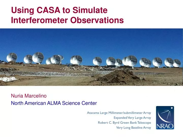
Using CASA to Simulate Interferometer Observations. Nuria Marcelino North American ALMA Science Center. Simulating Interferometer Data. Take a model image and simulate how it would look if observed by ALMA or the JVLA . Other arrays (e.g., SMA, CARMA, etc.) also included

E N D
Using CASA to Simulate Interferometer Observations • Nuria Marcelino • North American ALMA Science Center
Simulating Interferometer Data • Take a model image and simulate how it would look if observed by ALMA or the JVLA. • Other arrays (e.g., SMA, CARMA, etc.) also included • Explore the effects of: • Number of antennas • Antenna configuration • Length of observation • Thermal noise • Phase noise • Functionality included in CASA via tasks simobserveand simanalyze(nee simdata). • CASAguides includes several walkthroughs:http://casaguides.nrao.edu/index.php?title=Simulating_Observations_in_CASA
Basic Simulation Workflow Model Sky Distribution (FITS, image, components) In CASA… simobserve Simulated Measurement Set (calibrated u-v data) simanalyze Simulated Image & Analysis Plots Comparing “Observed”/original image
Simulation Tasks • simobservesimulates interferometric (and single dish)observations of a source. • simanalyzeimages and analyzes these simulations. “tasklist” output
simobserve • simulates interferometer observations of a source. “inpsimobserve” output
CASA Refresher • inpshows parameter names Expandable parameter(currently NOT expanded) Expandable parameter(currently expanded)
CASA Refresher • inpshows current value (change, e.g., by project = “myproj”) Invalid Value
CASA Refresher • inpshows current value (change, e.g., by project = “myproj”) ValidValue DefaultValue
CASA Refresher • inpshows brief description
CASA Refresher • When all parameters are set, execute with “go simobserve” • If you get stuck: • Type “tasklist” to see all tasks • Type “help taskname” to get help on taskname • Type “default taskname” to set the default inputs • Type “inp” to review the inputs of the current task • Ask!
Basic Simulation Workflow Model Sky Distribution (FITS, image, components) In CASA… simobserve Simulated Measurement Set (calibrated u-v data) simanalyze Simulated Image & Analysis Plots Comparing “Observed”/original image
What Defines a Simulation? Model Sky Distribution(Required) What does the sky really look like in your field? Telescope(Required) Number of Antennas, Configuration, Diameter Observation(Required) Integration time, scan length, pointing centers Corruption (Optional) Thermal noise, phase noise, polarization leakage
simobserve • Model sky distribution as FITS file or “component list” Model Sky Distribution(Required) What does the sky really look like in your field?
Input Sky Model • Model sky distribution as FITS file. simobserveneeds: • Coordinates • Brightness units • Pixel scale (angular and spectral) • Stokes axis (optional) • These may be specified in your FITS header or supplied/over-written by simobserve.
Input Sky Model • Alternatively, supply a Gaussian “component list.” • Example at:http://casaguides.nrao.edu/index.php?title=Simulation_Guide_Component_Lists_(CASA_3.3)
Simple Example • Simulate observing 1mm dust continuum in a 30-Doradus (LMC)-like region at the distance of M31/M33 (800 kpc). • We have a near-IR image of 30 Doradus, will need to: • Scale the brightness and observing frequency • Adjust the pixel scale(move it from 50-800 kpc) • Set a new position • Define the observationsintegration time, telescope, etc. Our Model 30 Doradus in the LMC 8 μm (credit: SAGE collaboration)
Simple Example • inbright = “0.6mJy/pixel”Requires spectral model/other knowledge to estimate (Science!) • Indirection = “J2000 10h00m00s -40d00m00s” • incell=“0.15arcsec”native cell size = 2.3”, moving from 50 kpc800 kpc scale by 50/800 • incenter=“230GHz”, inwidth=“2GHz”Need to supply observing frequency & bandwidth (here 1mm dust continuum)
Simple Example • inbright = “0.6mJy/pixel”Requires spectral model/other knowledge to estimate (Science!) • Indirection = “J2000 10h00m00s -40d00m00s” • incell=“0.15arcsec”native cell size = 2.3”, moving from 50 kpc800 kpc scale by 50/800 • incenter=“230GHz”, inwidth=“2GHz”Need to supply observing frequency & bandwidth (here 1mm dust continuum)
simobserve • Telescope via configuration file. Telescope(Required) Number of Antennas, Configuration, Diameter
Configuration Files • Define telescope array for simobserve. Config Files in CASA Already ALMA, JVLA, CARMA, SMA, etc. Example Config File: ALMA Cycle 1 ACA xyz diameter name
Configuration Files • Pick an intermediate-extent full-ALMA configuration
simobserve • Observations defined via setpointingsand obsmode Observation(Required) Integration time, scan length, pointing centers
setpointings • setpointingsdictates field, integration time, mosaic • integration sets data averaging (and field visit) timehere averaging 600s (10m) ensures a quick initial execution • direction sets field or map center • mapsize, maptype, pointingspacingdefine a mosaicBy default it will cover the model, here that means a 9-point mosaic
obsmode • obsmodesets total time, date, observing sequence • totaltimesets total observationtimeHere 7200s (2h) is the default value • Optionally specify the date, LST, and a calibrator sequence. go simobservesimobserve creates a measurement set (MS) in projectname/projectname.ms
skymodel image • simobserveoutputs several filesto project directory: • projectname.alma.out10.ms/ • projectname.alma.out10.observe.png • projectname.alma.out10.ptg.txt • Text files show the location of pointing centers • projectname.alma.out10.quick.psf • projectname.alma.out10.skymodel/ • projectname.alma.out10.skymodel.flat/ • projectname.alma.out10.skymodel.png
simobserve • Corruption with thermalnoise& toolkit Corruption (Optional) Thermal noise, phase noise, polarization leakage
thermalnoise • Set observing conditions to add random noise to image • ATM model specific for ALMA site ! • Use instead…
thermalnoise • Set observing conditions to add random noise to image • ATM model specific for ALMA site ! • See CASAguidesand toolkit manual for other ways to corrupt data. (e.g., phase noise) • http://casaguides.nrao.edu/index.php?title=Corrupt • http://casa.nrao.edu/docs/casaref/CasaRef.html (Simulator tool, sm) go simobservesimobserve creates a noisymeasurement set (MS) in projectname/projectname.noisy.ms
thermalnoise • Set observing conditions to add random noise to image • model no noise 3mm pwv
Multiple sets of observations • One can simulate multiple sets of observations with multiple calls to simobserve, to: • simulate combining datawith different hour angles • simulate combining data from different configurations (JVLA A+D), or arrays (ALMA 12m+ACA) • simulate combining data from interferometers and single dish telescopes (JVLA+GBT) • The CLEAN task can take multiple measurement sets to combine interferometricobservations • The FEATHER task can combine single dish and interferometric observations
Basic Simulation Workflow Model Sky Distribution (FITS, image, components) In CASA… simobserve Simulated Measurement Set (calibrated u-v data) simanalyze Simulated Image & Analysis Plots Comparing “Observed”/original image
simanalyze • Image and analyze simobserveoutput
image • Grid, invert, and CLEAN the simulated data set. • Similar but reduced options compared to CLEAN.Defaults are “smart”, informed by the model. • You can also image the simulated observations with CLEAN.They are a normal CASA measurement set for all purposes
image • Output files can be examined with the CASA viewer.In CASA 3.4 these live in projectname/projectname.image
analyze • Create diagnostic plots based on simobserveand image • Pick up to 6 of these. go simanalyzesimanalyzecreatesimages and diagnostic plotsin projectname/
analyze • Create diagnostic plots based on simobserveand image
analyze • Create diagnostic plots based on simobserveand image Point spread function Sky Model u-v coverage Simulated image Difference Image Fidelity
Try It Yourself! • Simulate one of the suite of model images at http://casaguides.nrao.edu/index.php?title=Sim_Inputs