Download
1 / 37
370 likes | 522 Views
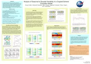
Coupled General Circulation Modeling. Anthony J. Broccoli Dept. of Environmental Sciences. Is There a Better Set of Lower Boundary Conditions?. Yes! The lower boundary conditions for the atmosphere could be determined interactively in response to processes internal to the model.

E N D
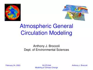
Coupled General Circulation Modeling Anthony J. BroccoliDept. of Environmental Sciences 16:375:544Modeling of Climate Change
Is There a Better Set of Lower Boundary Conditions? • Yes! The lower boundary conditions for the atmosphere could be determined interactively in response to processes internal to the model. • This goal can be achieved by coupling the atmosphere to an ocean model. 16:375:544Modeling of Climate Change
Today’s Lecture • Types of coupled models • Coupling methods • Climate drift • Flux correction/adjustment • Design of coupled model experiments 16:375:544Modeling of Climate Change
Types of Coupled Models • Atmosphere-swamp ocean • Atmosphere-mixed layer ocean • Atmosphere-ocean GCM • Earth system models of intermediate complexity (EMICs) 16:375:544Modeling of Climate Change
Atmosphere-Swamp Ocean • Ocean is represented as a wet surface with zero heat capacity. • Surface temperature is interactively determined. • Albedo of swamp surface increases when temperature falls below freezing. 16:375:544Modeling of Climate Change
Atmospheric GCM land swamp Atmosphere-Swamp Ocean 16:375:544Modeling of Climate Change
Atmosphere-Mixed Layer Ocean • Ocean is represented as a shallow, motionless slab of water. • Mixed layer depth is chosen to represent seasonal heat storage in upper ocean. • Ocean temperature is interactively determined. • Sea ice thermodynamics are included. 16:375:544Modeling of Climate Change
Atmospheric GCM land mixed layer ocean Atmosphere-Mixed Layer Ocean 16:375:544Modeling of Climate Change
Atmosphere-Ocean GCM • Ocean component is a full dynamical ocean model, including advection, diffusion, heat storage. • Relatively complete representation of physical and dynamical feedbacks between atmosphere and ocean. 16:375:544Modeling of Climate Change
Atmosphere-Ocean GCM Atmospheric GCM land cons. of momentum,cons. of mass,cons. of saltcons. of thermal energyequation of state 16:375:544Modeling of Climate Change
EMICs • EMICs: Earth System Models of Intermediate Complexity • Designed to contain many feedbacks of full AOGCM but consume far less computer time. • Used for climate simulations that require long time scales (i.e., >1000 years). 16:375:544Modeling of Climate Change
EMIC Example: Ocean GCM with Energy Balance Atmosphere • Developed by A. Weaver and collaborators at Univ. of Victoria. • OGCM is coupled to simple atmosphere. • Atmospheric dynamics represented by diffusion. • Highly simplified parameterization of atmospheric radiation. 16:375:544Modeling of Climate Change
Coupling Methods • Communication between components is an essential element of coupled models. • Model component codes are often developed separately, so grids can be different, making regridding necessary. • Frequency of communication must be managed, particularly given the difference in response times of atmosphere and ocean. 16:375:544Modeling of Climate Change
Atmospheric model Couplinginterface Wind stressP-EHeat flux Surface temperatureAlbedo Sea ice model Couplinginterface Temperature SalinityOcean currents StressFresh water fluxHeat flux Ocean model Coupling Methods: Example 16:375:544Modeling of Climate Change
Asynchronous Coupling • Atmosphere is run for a relatively short period with output archived in “library.” • Ocean is run (with acceleration methods) for relatively long period using fluxes from atmospheric library. • Cycle can be repeated indefinitely. 16:375:544Modeling of Climate Change
Synchronous Coupling • Conceptually simple; no acceleration techniques are used. • Model components may have different time steps, but communication occurs at a fixed interval. • Typical interval: 1x daily (models without diurnal variation); 8x daily (with diurnal variation) 16:375:544Modeling of Climate Change
Climate Drift • Coupled models are typically constructed from atmosphere and ocean components that have been independently developed. • Stand-alone atmosphere and ocean components are tightly constrained by observed boundary conditions. • When atmosphere and ocean components are coupled, the resulting climate will often drift away from a realistic state. 16:375:544Modeling of Climate Change
Climate Drift in GFDL CM2 Zonal Mean SST Error from CM2_a10o2 [K] 16:375:544Modeling of Climate Change
Causes of Climate Drift Flux Difference [W m-2]AGCM vs. OGCM CM2_a10o2 SST Error [K] 16:375:544Modeling of Climate Change
Causes of Climate Drift • Imbalances between atmosphere-ocean heat fluxes simulated by AGCM and OGCM when both are run with observed SSTs. • Climate feedbacks triggered by flux imbalances. (Ex: CM2_a10o2 cooling pattern in midlatitude N.H. → southward shift in westerlies → error in position of western boundary currents) 16:375:544Modeling of Climate Change
Flux Corrections/Adjustments • One ad hoc approach to reducing climate drift is to adjust for differences in atmospheric and oceanic component fluxes by adding a compensating flux at each grid point. • This method is known as flux correction (Sausen et al. 1986) or flux adjustment (Manabe et al. 1991). 16:375:544Modeling of Climate Change
Calculating Flux Adjustments • The goal is to determine artificial heat and water fluxes that vary seasonally and spatially but do not depend on the state of the model. • Method 1: GFDL Three-Step • Method 2: Coupled Restore • Method 3: Offline Flux Difference 16:375:544Modeling of Climate Change
Method 1: GFDL Three-Step • Step 1: Run the AGCM with climatological SSTs, archiving the heat and water fluxes. • Step 2: Run the OGCM with the fluxes from step 1, while simultaneously restoring to observed T and S. 16:375:544Modeling of Climate Change
Method 1: GFDL Three-Step • Step 1: Run the AGCM with climatological SSTs, archiving the heat and water fluxes. • Step 2: Run the OGCM with the fluxes from step 1, while simultaneously restoring to observed T and S. Restoring terms 16:375:544Modeling of Climate Change
Method 1: GFDL Three-Step • Step 1: Run the AGCM with climatological SSTs, archiving the heat and water fluxes. • Step 2: Run the OGCM with the fluxes from step 1, while simultaneously restoring to observed T and S. • Step 3: Couple the AGCM and OGCM without restoring, using the archived restoring terms from step 2 as flux adjustments. 16:375:544Modeling of Climate Change
Method 2: Coupled Restore • Step 1: Couple the AGCM and OGCM, then run the coupled models while simultaneously restoring to observed T and S, archiving the restoring terms as flux adjustments. • Step 2: Deactivate the restoring and run the coupled AOGCM using the flux adjustments determined in step 1. 16:375:544Modeling of Climate Change
Method 3: Offline Flux Differences • Step 1: Run the AGCM with climatological SSTs, archiving the heat and water fluxes. • Step 2: Run the OGCM, restoring to observed T and S. Archive the restoring fluxes. • Step 3: The differences between the fluxes from step 1 and step 2 are the flux adjustments; these are supplied to the coupled AOGCM. 16:375:544Modeling of Climate Change
Flux Adjustment: Pros and Cons Cons • Flux adjustments are nonphysical. • There is no guarantee that coupled model biases are invariant over different climate states. • Flux adjustments could distort climate feedbacks. 16:375:544Modeling of Climate Change
Flux Adjustment: Pros and Cons Pros • Flux adjustments minimize climate drift that would distort climate feedbacks if left unchecked. • Flux adjustments allow sensitivity experiments to be performed while better models (i.e., those with smaller errors) are under development. 16:375:544Modeling of Climate Change
Design of Coupled Model Experiments • Equilibrium: The goal is to determine the climate that is in equilibrium with a given set of climate forcings. (Example: What climate state is in equilibrium with twice the preindustrial level of atmospheric CO2?) • Transient: The goal is to investigate the time-dependent response of the climate to a given (often time-dependent) change. (Example: How will the climate change in response to projected increases in CO2 and other human-induced climate forcings?) 16:375:544Modeling of Climate Change
Types of Experiments • Forcing-Response: Impose a specific forcing and see how the model responds. • Unforced Variability: Allow a model to run, preferably for a lengthy period, and examine the spatiotemporal variations that are generated by the internal dynamics of the model. 16:375:544Modeling of Climate Change
Design of Coupled Model Experiments: Issues • Initialization: How to Start? • Equilibration: How Long to Run? • Fidelity: How Good is the Model? 16:375:544Modeling of Climate Change
Initialization • Not typically an important issue for atmosphere-only or atmosphere-mixed layer ocean models. • More important for AOGCMs; these can exhibit considerable sensitivity to initial conditions. • Issue:How to initialize time-dependent AOGCM simulations of past climates? 16:375:544Modeling of Climate Change
Equilibration • Time required varies with model type and depends on e-folding time of slowest component of climate system. • AGCMs: < 1 year • A-MLO models: ~5 years • AOGCMs: ~500-1,000 years 16:375:544Modeling of Climate Change
Equilibration • Integration length must be adequate for sampling climate statistics. • Acceleration techniques may be useful in ocean-only simulations, but should be used with caution. 16:375:544Modeling of Climate Change
Fidelity • How well does a model simulate the important processes of interest? • Careful comparison of model simulations with the observed climate record are critical for assessments of model fidelity. • Successful performance in such comparisons can increase our confidence in climate models. 16:375:544Modeling of Climate Change
Friday’s Seminar Date: February 28 Time: 2:00 PM Place: ENRS Building, Room 223Title: "The New GFDL Global Atmosphere and Land Model AM2/LM2"Speaker:Dr. Stephen Klein, NOAA/GFDL 16:375:544Modeling of Climate Change