Download
1 / 33
430 likes | 955 Views
ArrayComm Presentation. Semi-Blind (SB) Multiple-Input Multiple-Output (MIMO) Channel Estimation. Aditya K. Jagannatham DSP MIMO Group, UCSD. Overview of Talk. Semi-Blind MIMO flat-fading Channel estimation. Motivation Scheme: Constrained Estimators.

E N D
ArrayComm Presentation Semi-Blind (SB) Multiple-Input Multiple-Output (MIMO) Channel Estimation Aditya K. Jagannatham DSP MIMO Group, UCSD
Overview of Talk • Semi-Blind MIMO flat-fading Channel estimation. • Motivation • Scheme: Constrained Estimators. • Construction of Complex Constrained Cramer Rao Bound (CC-CRB). • Additional Applications: Time Vs. Freq. domain OFDM channel estimation. • Frequency selective MIMO channel estimation. • Fisher information matrix (FIM) based analysis • Semi-blind estimation.
Rx r- receive TX t - transmit Receiver Transmitter =Antenna MIMO System Model • A MIMO system is characterized by multiple transmit (Tx) and receive (Rx) antennas • The channel between each Tx-Rx pair is characterized by a Complex fading Coefficient • hijdenotes the channel between theithreceiver and jth transmitter. • This channel is represented by the Flat-Fading Channel MatrixH
MIMO System H MIMO System Model where, is the r x t complex channel matrix • Estimating H is the problem of ‘Channel Estimation’ • #Parameters = 2.r.t (real parameters)
MIMO Channel Estimation • CSI (Channel State Information) is critical in MIMO Systems. - Detection, Precoding, Beamforming, etc. • Channel estimation holds key to MIMO gains. • As the number of channels increases, employing entirely training data to learn the channel would result in poorer spectral efficiency. - Calls for efficient use of blind and training information. • As the diversity of the MIMO system increases, the operating SNR decreases. - Calls for more robust estimation strategies.
H(z) Training inputs Training outputs Outputs Inputs Training Based Estimation • One can formulate the Least-Squares cost function, • The estimate of H is given as • Training symbols convey no information.
H(z) ‘Blind’ data inputs ‘Blind’ data outputs Blind Estimation • Uses information in source statistics. • Statistics: - Source covariance is known,E(x(k)x(k)H) = σs2It - Noise covariance is known, E(v(k)v(k)H) = σn2Ir • Estimate channel entirely from blind information symbols. • No training necessary.
Training Blind Channel Estimation Schemes • Is there a way to trade-off BW efficiency for algorithmic simplicity and complete estimation. • How much information can be obtained from blind data? • In other words, how many of the 2rt parameters can be estimated blind ? • How does one quantify the performance of an SB Scheme ? Increasing Complexity Decreasing BW Efficiency
Semi-Blind Estimation N symbols • Training information - Xp = [x(1), x(2),…, x(L)] ,Yp = [y(1), y(2),…, y(L)] • Blind information - E (x(k)x(k)H) = σs2It, E (v(k)v(k)H) = σn2Ir • (N-L),the number of blind “information” symbols can be large. • L, the pilot length is critical. H(z) Training inputs ‘Blind’ data inputs Training outputs ‘Blind’ data outputs
Whitening-Rotation • His decomposed as a matrix product,H= WQH. • For instance, if SVD(H) = P QH, W = P. Wis known as the “whitening” matrix Wcan be estimated using only ‘Blind’ data. H= WQH QQH = I Qis a ‘constrained’ matrix Q , the unitary matrix, cannot be estimated from Second Order Statistics.
Estimating Q • How to estimateQ ? • Solution : EstimateQfrom the training sequence ! Advantages Unitary matrixQparameterized by a significantly lesser number of parameters thanH. r x r unitary - r2 parameters r x r complex - 2r2 parameters • As the number of receive antennas increases, sizeofHincreases while that ofQremains constant • size of H is r x t • size of Q is t x t
Estimating W • Output correlation : • Estimate output correlation • EstimateW by a matrix square root (Cholesky) factorization as, • As # blind symbols grows ( i.e. N ), . • AssumingWis known, it remains to estimateQ.
Constrained Estimation • Orthogonal Pilot Maximum Likelihood – OPML • Goal - Minimize the ‘True-Likelihood’ subject to : • Estimate: • Properties 1. Achieves CRB asymptotically in pilot length, L. 2. Also achieves CRB asymptotically in SNR.
p(;) parameter Observations Parameter Estimation • Estimator : • For instance - Estimation of the mean of a Gaussian • Estimator
Cramer-Rao Bound (CRB) • Performance of an unbiased estimator is measured by its covariance as • CRB gives a lower bound on the achievable estimation error. • The CRB on the covariance of an un-biased estimator is given as where
CRB Complex Cons. Par. Estimator Constrained Estimation • Most literature pertains to “unconstrained-real” parameter estimation. • Results for ‘complex’ parameter estimation ? • What are the corresponding results for “constrained” estimation? • For instance, estimation of a unit norm constrained singular vector i.e.
p(, )be thelikelihoodof the observationparameterized by Define the extended parameter vector as With complexderivatives, define the matrixF ()as Define the extended constraint setf () Uspan the NullSpace ofF(). Complex-Constrained Estimation • Builds on work by Stoica’97 and VanDenBos’93 Letbe ann- dim constrained complex parameter vector The constraints onare given byh( ) = 0
Jis the complex un-constrained Fischer Information Matrix (FIM) defined as CRB Result : The CRB for the estimation of the ‘complex-constrained’ parameter is given as Constrained Estimation(Contd.)
Semi-Blind CC-CRB • LetQ = [q1, q2,…., qt].qiis thus a column ofQ . The constraints onqisare given as: • Unit norm constraints:qiHqi = ||qi||2 = 1 • Orthogonality Constraints :qiHqj = 0 for i j • Constraint Matrix : • Let SVD( H )be given asP QH. • CRB on the variance of the(k,l)thelement is
Unconstrained Parameters • has only‘n’un-constrained parameters, which can vary freely. • has only(n = )1 un-constrained parameter. • t x t complex unitary matrix Q has only t2un-constrained parameters. • Hence, ifWis known,H = WQH hast2un-constrained parameters.
Semi-Blind CRB • LetNbe the number of un-constrained parameters inH. • Also, Xpbe an orthogonal pilot.i.e.Xp XpHI • Estimation is directly proportional to the number of un-constrained parameters. • E.g. For an8 X 4complex matrixH, N= 64. The unitary matrixQis 4 X 4and hasN= 16parameters. Hence, the ratio of semi-blind to training based MSE of estimation is given as
Simulation Results • Perfect W, MSE vs. L. • r = 8, t = 4.
OFDM Channel Estimation • Time Vs. Freq. Domain channel estimation for OFDM systems. • Consider a multicarrier system with # channel taps = L (10), # sub-carriers = K(32,64) • h is the channel vector. • g = Fsh,whereFs is the leftK x Lsubmatrix ofF (Fourier Matrix). • Total # constrained parameters =K(i.e. dim. of H ). • # un-constrained parameters =L(i.e. dim. of h ).
x(k) D D D + + + H(0) H(1) H(2) H(L-1) y(k) FIR-MIMO System • H(0),H(1),…,H(L-1) to be estimated. • r = #receive antennas, t = #transmit antennas (r > t). • #Parameters = 2.r.t.L (L complex r X t matrices)
Fisher Information Matrix (FIM) • Let p(ω;θ) be the p.d.f. of the observation vector ω. • The FIM (Fisher Information Matrix) of the parameter θ is given as • Result: Rank of the matrix Jθequal to the number of identifiable parameters. • In other words, the dimension of its null space is precisely the number of un-identifiable parameters.
SB Estimation for MIMO-FIR • FIM based analysis yields insights in to SB estimation. • Letthe channel be parameterized as θ2rtL. • Application to MIMO Estimation: • Jθ = JB + Jt, where JB, Jt are the blind and training CRBs respectively. • It can then be demonstrated that for irreducible MIMO-FIR channels with (r >t), rank(JB) is given as
Implications for Estimation • Total number of parameters in a MIMO-FIR system is 2.r.t.L . However, the number of un-identifiable parameters is t2. • For instance, r = 8, t = 2, L = 4. • Total #parameters = 128. • # blindly unidentifiable parameters = 4. • This implies that a large part of the channel, can be identified blind, without any training. • How does one estimate the t2 parameters ?
Semi-Blind (SB) FIM • The t2 indeterminate parameters are estimated from pilot symbols. • How many pilot symbols are needed for identifiability? • Again, answer is found from rank(Jθ). • Jθ is full rank for identifiability. • If Lt is the number of pilot symbols, • Lt =t for full rank, i.e. rank(Jθ) = 2rtL.
SB Estimation Scheme • The t2 parameters correspond to a unitary matrix Q. • H(z) can be decomposed as H(z) = W(z) QH. • W(z) can be estimated from blind data [Tugnait’00] • The unitary matrix Q can be estimated from the pilot symbols through a ‘Constrained’ Maximum-Likelihood (ML) estimate. • Let x(1), x(2),…,x(Lt) be the Lttransmitted pilot symbols.
Semi-Blind CRB • Asymptotically, as the number of data symbols increases, semi-blind MSE is given as • Denote MSEt = Training MSE, MSESB = SB MSE. • MSESB α t2 (indeterminate parameters) • MSEt α2.r.t.L (total parameters). • Hence the ratio of the limiting MSEs is given as
Simulation • r = 4, t = 2 (i.e. 4 X 2 MIMO system). L = 2 Taps. • Fig. is a plot of MSE Vs. SNR. • SB estimation is 32/4 i.e. 9dB lower in MSE
Talk Summary • Complex channel matrix H has 2rt parameters. • Training based scheme estimates 2rt parameters. • SB scheme estimates t2 parameters. • From CC-CRB theory, MSE α #Parameters. • Hence, • FIR channel matrix H(z) has 2rtL parameters. • Training scheme estimates 2rtL parameters. • From FIM analysis, only t2 parameters are unknown. • Hence, SB scheme can potentially be very efficient.
References Journal • Aditya K. Jagannatham and Bhaskar D. Rao, "Cramer-Rao Lower Bound for Constrained Complex Parameters", IEEE Signal Processing Letters, Vol. 11, no. 11, Nov. 2004. • Aditya K. Jagannatham and Bhaskar D. Rao, "Whitening-Rotation Based Semi-Blind MIMO Channel Estimation" - IEEE Transactions on Signal Processing, Accepted for publication. • Chandra R. Murthy, Aditya K. Jagannatham and Bhaskar D. Rao, "Semi-Blind MIMO Channel Estimation for Maximum Ratio Transmission" - IEEE Transactions on Signal Processing, Accepted for publication. • Aditya K. Jagannatham and Bhaskar D. Rao, “Semi-Blind MIMO FIR Channel Estimation: Regularity and Algorithms”, Submitted to IEEE Transactions on Signal Processing.