Download
1 / 22
270 likes | 667 Views
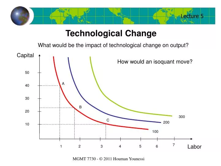
Technological Change. What would be the impact of technological change on output?. Capital. How would an isoquant move?. 50. A. 40. 30. B. 20. 300. C. 200. 10. 100. 7. Labor. 1. 2. 3. 4. 5. 6. But productivity can increase without technological change!.

E N D
Technological Change What would be the impact of technological change on output? Capital How would an isoquant move? 50 A 40 30 B 20 300 C 200 10 100 7 Labor 1 2 3 4 5 6
But productivity can increase without technological change! Note however, that we are NOT producing more Capital K C2 C Q C1 B B’ I A’ C’ A Labor L1 L2
Total Factor Productivity A Better Measure for Technological Change Total factor productivity measure, relates changes in output to all inputs. In the case of our example to labor AND capital. Take for instance a production function: Where Q is the quantity of output, L is quantity of labor, b is a labor related rate, c is a capital related rate such as unit price (both constants) We divide the quantity by the sum of all the weighted inputs to get a ratio α In general: Where wi is the weight associated with the ith input Ii
Cost • Historical cost • Opportunity cost • Explicit cost • Implicit cost • Short-run cost • Long-run cost
Historical V Opportunity Cost Historical cost: The amount – in currency – that the entity paid for a good or service (The “I don’t believe I paid for that” cost) Opportunity cost: The value of the highest valued good or service you could have procured if you had not selected the present option (The “I could have had a V8” cost)
Explicit V Implicit Cost Explicit Cost: Ordinary items that accountants include as accountable costs, e.g. payroll, cost of materials, etc. Implicit Cost: The hidden –usually unaccounted for – charges, e.g. owner’s time
Short-run V Long-run Cost Function Short-run: The immediate time frame during which the entity (firm) cannot change the quantity of at least some of the inputs. Long-run: The time frame during which the entity (firm) has had time to adjust to give itself the ability to change the quantity of at least one of the inputs.
Short-run Cost Function As the firm is unable to alter the quantities of some inputs such as plant and equipment – or sometimes even labor – short run functions are characterized by: Fixed costs Total cost (TC) Cost Cost As well as, of course, Total variable cost (TVC) Total variable cost (TVC) Variable costs Total fixed cost (TFC) Total fixed cost (TFC) Total cost in the short-run is therefore: TC=TFC+TVC Output Output
Average and Marginal Cost Average fixed cost (AFC): is total fixed cost per unit of output (and it DOES change!) Average variable cost (AVC): is total variable cost per unit of output Average total cost (ATC): the sum of the two, or total cost per unit of output
Cost Marginal Cost=dTC/dQ Average Total Cost Average Variable Cost Average Fixed Cost Output
Marginal Cost The addition to total cost resulting from the addition of the last unit of output We know that TVC is the product of the price of the variable unit (W) and the quantity of variable input (U) We also know that the change of the variable input U wrt quantity is the marginal product of that variable input So what variable price W should you pay for your input (say some raw material)?
Example: ABCO has a total cost function as below: The firm’s marginal cost function will be: The firm’s average variable cost function will be: Note that marginal cost always equals average variable cost when AVC is at a minimum.
Note also that marginal cost always equals average total cost when ATC is at a minimum.
Long-run Cost Function In the long-run, the organization has had the time to adjust, may be expand equipment capacity, install new equipment, open a new plan or catch up with technology. Nothing – no input – is frozen and the organization can PLAN for a new set of future short-run situations. Imagine…… that an organization wishes to expand output. Let us say, it has the choice of opening three types of plants – three years from now. The short-run average cost function for each plant is given Average Cost C1 C2 C3 Output Quantity
Average Cost C1 C2 C3 Q2 Q1 Output Quantity
Average Cost Long-run Average Cost Function Short-run Average Cost Functions Output Quantity
Given the long-run average cost, we can calculate the long-run total cost: Given the long-run total cost, we can calculate the long-run marginal cost:
Example: Ephemer Industries has the production function: As Ephemer pays $8 for hour of labor and $2 for unit of capital, it’s total cost is: In the short-run K is fixed at K=10, thus: Where TCS is short-run total cost. Short-run Average Cost will be:
And the short-run marginal cost is: In the long-run, in input is fixed. We wish to determine the optimum amount of capital input to be used to produce Q units per months, we minimize the total cost function Substituting, we have This implies that the long-run average cost equals $2 per unit produced.
Economies of Scope Economies of scope exist when the cost of producing two (or more) products jointly is less than the sum cost of producing each one alone To determine if economies of scope are available to us, we calculate: S represents the percent savings due to economies of scope
Break-Even Analysis Profit ensues when all costs are covered Break-even analysis will find the point where total cost and total revenue are equal $ Total Cost Total Revenue Quantity
Example: Makeabuck Inc. has the total cost function: The firm’s total revenue is: How many units of product must the firm will make and sell to start making a profit ?