Introduction to FLUID DYNAMICS

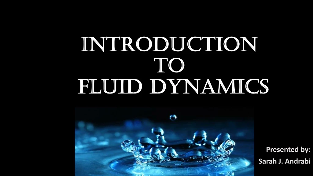
1. Introduction toFLUID DYNAMICS Presented by: Sarah J. Andrabi

2. Outline • Introduction • Fluid Characteristics • Challenges • Mathematical Review • Navier-Stokes Equations • Different Techniques—Lagrangainand Eulerian • Building a 2D simulator • Solid-Fluid interaction • Open Issues • References https://www.youtube.com/watch?v=DxawCFRSwts

3. Introduction • So many fluids in our surroundings • Realistic animations of water, smoke, explosions, fire and related phenomena • Evolve the motion of the fluid forward in time • Describe the physics of the fluids

4. Motivation • Applications • Games • Medical simulation (Blood flow, etc) • Movie special effects (Interstellar, Pirates of the Caribbean) • Scientific visualization (Water sewage system, dam construction)

5. Fluid Characteristics • Basic properties • Pressure • Viscosity • Surface tension • Density

6. Fluid Characteristics • Types of Fluids • Compressible fluids: Change in density is significant with changes in pressure and temperature • Incompressible fluids: Change in density with change in pressure and temperature is not significant • Viscous fluids: Resist deformation • Inviscid fluids: No viscosity

7. Fluid Characteristics • Types of Fluids • Turbulent:Flow that appears to have chaotic and random changes • Laminar (streamline) flow: Flow that has smooth behavior • Newtonian fluids: Fluids continue to flow, regardless of the force acting on it • Non-Newtonian fluids: Fluids that have non-constant viscosity • Phase Transition— Fluids may change physical behavior under different environmental conditions

8. Challenges in Fluid Simulation • Modeling continuum fluids on discrete systems – It’s all about approximations • Topological variations and different kinds of behaviors with interacting subjects • Numerical stabilities, accuracy and convergence issues • Performance • User control

9. Mathematical Review • Gradient (of a scalar field): , is a vector field • Describes how the scalar field changes spatially • Divergence:, is the dot product of the gradient with a vector • Describes the net flow out of or into points in the vector field • Laplacian:, is the dot product of two gradient operators • Describes how much values in the original field differ from their neighborhood average

10. Navier-Stokes Equations • Describe the velocity field of a fluid, u, over time • Set of two equations • First equation—says that the amount of fluid flowing into any volume must be equal to the amount of fluid flowing out • “Incompressibility equation” • Second equation—Accounts for motion of fluid through space, accounting for internal or external forces

11. Navier-Stokes Equations • Derivative of velocity w.r.t. time—how fluid accelerates due to forces acting on it Change in velocity Diffusion/Viscosity Advection Pressure Body Forces

12. Navier-Stokes Equations • Kinematic Viscosity –determines thickness of fluid • How much the fluid resists deformation while flowing • Acts as a force that tries to make our particle move at the average velocity of the nearby particles Change in velocity Diffusion/Viscosity Advection Pressure Body Forces

13. Navier-Stokes Equations • Convection (or advection)—arises due to conservation of momentum • Think of it as the momentum moving or ‘convecting’ through space along with the fluid Change in velocity Diffusion/Viscosity Advection Pressure Body Forces

14. Navier-Stokes Equations • Captures forces generated by pressure differences within the fluid • is the density of the fluid • - captures the imbalance in pressure at a specific position Change in velocity Diffusion/Viscosity Advection Pressure Body Forces

15. Navier-Stokes Equations • Includes external forces like gravity or contact forces Change in velocity Diffusion/Viscosity Advection Pressure Body Forces

16. Techniques Overview • Common techniques for solving Navier-Stoke’s equation: • Eulerian approach (grid-based) • Lagrangian approach (particle-based) • Spectral method • Lattice Boltzmann method [Stam] Stable Fluids, SIGGRAPH 99 [Mueller, Charypar, Gross] Particle-Based Fluid Simulation for Interactive Applications, SCA03

17. Lagrangian vs. Eulerian in One Picture

18. Lagrangian Approach • Treat fluids like a particle system • Each particle has a position and a velocity • Discrete set of particles usually connected up in a mesh • Solids are almost always simulated in this way • Evaluation: • Mass / Momentum conservation • More intuitive • Faster • Need space partition structure for connectivity information • Need for surface reconstruction

19. Eulerian Approach • No particle tracking • Corresponds to a fixed grid that doesn’t change in space even as the fluid flows through it • Look at specific points in space and see how at those points the fluid quantities change over time • Used mostly for fluids • Evaluation: • Derivative approximation is easier • Adaptive time step/solver • Memory usage & speed • Grid artifact/resolution limitation to capture fluid detail

20. Lagrangian vs. Eulerian Lagrangian • http://www.youtube.com/watch?v=6CP5QvfuD_w Eulerian • http://www.youtube.com/watch?v=Jl54WZtm0QE

21. Case Study: A 2D Fluid Simulator • Focus on incompressible, viscous fluid • Consider gravity as the only external force • No inflow or outflow • Constant viscosity, constant density everywhere in the fluid

22. Simulation Loop Diffusion Advection Body Force Scalar/Vector fields defined on the grid Pressure Solve ut = 2u –(u)u – p + u=0

23. The Power of Operator Splitting • One complicated Multi-dimensional operator => A series of simple, lower dimensional operators • Each operator can have its own integration scheme and different time step sizes • High modularity and easy to debug Un + A + B + D + P U* U** U*** Un+1

24. Advection • Sometimes called “Convection” or “Transport” • Define how a quantity moves with the underlying velocity field • This term ensures the conservation of momentum • Advection equation: • Approaches: • Forward Euler (unstable) • Semi-Lagragian advection (stable for large time steps, but suffers from the dissipation issue)

25. Advection Forward Euler Advection Semi-Lagragian Advection

26. Diffusion • Define how a quantity in a cell inter-changes with its neighbors • Diffusion = Blurring Low Viscosity High Viscosity Figures from [Carlson, Mucha, Turk] Melting and Flowing, SCA 02

27. Diffusion • Diffusion equation: • Approaches: • Explicit formulation • Implicit formulation (for high viscosity) 1 1 -4 1 1 Unknowns

28. Diffusion 0 0 0 2.5 0 0 0 5 0 0 2.5 -10 0 2.5 0 0 0 0 0 0 2.5 0 Before the diffusion After the diffusion (k = 0.5, time step size =1)

29. Pressure Solve • It’s sometimes called “Pressure Projection” • What does the pressure do? • Keep the fluid at constant volume (incompressible, conservation of mass). • Make sure the velocity field stays divergence-free Incompressible Compressible

30. Pressure Solve • Equation to solve: • How to solve for pressure: • Taking divergence of both sides of (1) we get • Build a system of equations and solve using an iterative method such as Conjugate Gradient • Update the velocity field from the pressure gradient s.t. Unknowns • • • (1) (Poisson Equation)

31. Fluid-Solid Interaction • The fluid shouldn’t be flowing into and out of the solid • Consider velocity and pressure of the fluids as interacting with the solid • Consider boundary conditions— • Free surface • Fluid in contact with a solid wall container • Boundary between fluids Free surface Solid wall

32. Fluid-Solid Interaction • Pressure—makes fluid incompressible and “enforces solid wall boundary conditions” • Velocity at Boundary • Fluid needs to stay in • (if the solid isn’t moving) • Generally, Free surface “No-Stick” condition Solid wall

33. Fluid-Solid Interaction • Viscosity—Makes life a bit more harder • Simplest case for boundary condition: • (if solid isn’t moving) • (if solid is moving) • What if the wall is a vent or drain—the fluid needs to flow through https://www.youtube.com/watch?v=DxawCFRSwts “No-Slip” condition

34. What’s next… • 3D, Real-time and large scale scene fluid simulations • Hybrid techniques • http://www.youtube.com/watch?v=-HzNa2PB4b0&list=UU0GpuO2aEbGMG8N0iLE9_TA • Memory savings and speed ups • Fluid Simulations on other planets, in space etc

35. References • R. Bridson and M. Müller-Fischer. Fluid Simulation. SIGGRAPH 07 Course Notes • David Cline, David Cardon and Parris K. Egbert. Fluid Flow for the Rest of Us: Tutorial of the Marker and Cell Method in Computer Graphics • Stam, Jos. "Stable fluids." Proceedings of the 26th annual conference on Computer graphics and interactive techniques. ACM Press/Addison-Wesley Publishing Co., 1999. • Chentanez, Nuttapong, and Matthias Müller. "Real-time Eulerian water simulation using a restricted tall cell grid." ACM Transactions on Graphics (TOG). Vol. 30. No. 4. ACM, 2011. • http://www.youtube.com/watch?v=Jl54WZtm0QE • Müller, Matthias, David Charypar, and Markus Gross. "Particle-based fluid simulation for interactive applications." Proceedings of the 2003 ACM SIGGRAPH/Eurographics symposium on Computer animation. Eurographics Association, 2003. • http://www.youtube.com/watch?v=6CP5QvfuD_w • Fluids presentation by Micheal Su • Golas, Abhinav, et al. "Large-scale fluid simulation using velocity-vorticity domain decomposition." ACM Transactions on Graphics (TOG) 31.6 (2012): 148. • Water of “Battleship”, https://www.youtube.com/watch?v=DxawCFRSwts