Download
1 / 21
210 likes | 402 Views
Routing Algorithms. Raj Jain Professor of CIS The Ohio State University Columbus, OH 43210 Jain@cse.ohio-state.edu This presentation is available on-line at: http://www.cse.ohio-state.edu/~jain/cis677-98/. Routing algorithms Dykstra’s Algorithm Bellman Ford Algorithm ARPAnet routing.

E N D
Routing Algorithms Raj Jain Professor of CIS The Ohio State UniversityColumbus, OH 43210Jain@cse.ohio-state.eduThis presentation is available on-line at: http://www.cse.ohio-state.edu/~jain/cis677-98/
Routing algorithms • Dykstra’s Algorithm • Bellman Ford Algorithm • ARPAnet routing Overview
Routing Fig 9.5
Rooting or Routing • Rooting is what fans do at football games, what pics do for truffles under oak trees in the Vaucluse, and what nursery workers intent on propagation do to cuttings from plants. • Routing is how one creates a beveled edge on a table top or sends a corps of infanctrymen into full scale, disorganized retreat Ref: Piscitello and Chapin, p413
Routeing or Routing • Routeing: British • Routing: American • Since Oxford English Dictionary is much heavier than any other dictionary of American English, British English generally prevalis in the documents produced by ISO and CCITT; wherefore, most of the international standards for routing standards use the routeing spelling. Ref: Piscitello and Chapin, p413
Routing Techniques Elements • Performance criterion: Hops, Distance, Speed, Delay, Cost • Decision time: Packet, session • Decision place: Distributed, centralized, Source • Network information source: None, local, adjacent nodes, nodes along route, all nodes • Routing strategy: Fixed, adaptive, random, flooding • Adaptive routing update time: Continuous, periodic, topology change, major load change
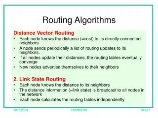
Distance Vector vs Link State • Distance Vector: Each router sends a vector of distances to its neighbors. The vector contains distances to all nodes in the network.Older method. Count to infinity problem. • Link State: Each router sends a vector of distances to all nodes. The vector contains only distances to neighbors. Newer method. Used currently in internet.
Dijkstra’s Algorithm • Goal: Find the least cost paths from a given node to all other nodes in the network • Notation: dij = Link cost from i to j if i and j are connectedDn = Total path cost from s to nM = Set of nodes so far for which the least cost path is known • Method: • Initialize: M={s}, Dn = dsn • Find node w M, whose Dn is minimum • Update Dn
M D2 Path D3 Path D4 Path D5 Path D6 Path 1 {1} 2 1-2 5 1-3 1 1-4 - - 2 {1,4} 2 1-2 4 1-4-3 1 1-4 2 1-4-5 - 3 {1,2,4} 2 1-2 4 1-4-3 1 1-4 2 1-4-5 - 4 {1,2,4,5} 2 1-2 3 1-4-5-3 1 1-4 2 1-4-5 4 1-4-5-6 5 {1,2,3,4,5} 2 1-2 3 1-4-5-3 1 1-4 2 1-4-5 4 1-4-5-6 6 {1,2,3,4,5,6} 2 1-2 3 1-4-5-3 1 1-4 2 1-4-5 4 1-4-5-6 Example (Cont) Table 9.4a
Bellman-Ford Algorithm • Notation:h = Number of hops being consideredD(h)n = Cost of h-hop path from s to n • Method: Find all nodes 1 hop away Find all nodes 2 hops away Find all nodes 3 hops away • Initialize: D(h)n = for all n s; D(h)n = 0 for all h • Find jth node for which h+1 hops cost is minimum D(h+1)n = minj [D(h)j +djn]
Example Fig 9.23b
Example (Cont) (h2) (h3) (h4) (h6) Path D (h5) h D Path D Path D Path D Path 0 - - - - - 1 2 1-2 5 1-3 1 1-4 - - 2 2 1-2 4 1-4-3 1 1-4 2 1-4-5 10 1-3-6 3 2 1-2 3 1-4-5-3 1 1-4 2 1-4-5 4 1-4-5-6 4 2 1-2 3 1-4-5-3 1 1-4 2 1-4-5 4 1-4-5-6 Table 9.4b
Flooding Fig 8.11b
Flooding • Uses all possible paths • Uses minimum hop path Used for source routing Fig 9.7
ARPAnet Routing (1969-78) • Features: Cost=Queue length, • Each node sends a vector of costs (to all nodes) to neighbors. Distance vector • Each node computes new cost vectors based on the new info using Bellman-Ford algorithm
ARPAnet Routing Algorithm Fig 9.9
ARPAnet Routing (1979-86) • Problem with earlier algorithm: Thrashing (packets went to areas of low queue length rather than the destination), Speed not considered • Solution: Cost=Measured delay over 10 seconds • Each node floods a vector of cost to neighbors.Link-state. Converges faster after topology changes. • Each node computes new cost vectors based on the new info using Dijkstra’s algorithm Fig 9.10
ARPAnet Routing (1987+) • Problem with 2nd Method: Correlation between delays reported and those experienced later : High in light loads, low during heavy loads Oscillations under heavy loads Unused capacity at some links, over-utilization of others, More variance in delay more frequent updates More overhead Fig 9.11
Routing Algorithm • Delay is averanged over 10 s • Link utilization = r = 2(s-t)/(s-2t)where t=measured delay, s=service time per packet (600 bit times) • Exponentially weighted average utilizationU(n+1) = U(n)+(1-)r(n+1) =0.5 U(n)+0.5 r(n+1) with = 0.5 • Link cost = fn(U) Fig 9.12
Summary • Distance Vector and Link State • Routing: Least-cost, Flooding, Adaptive • Dijkstra’s and Bellman-Ford algorithms • ARPAnet