Download
1 / 40
510 likes | 2.49k Views
Radar Project Pulse Compression Radar. By: Hamdi M. Joudeh and Yousef Al-Yazji Supervisor: Dr. Mohamed Ouda. Introduction:. Radars can be classified according to the waveforms: - Continuous Wave (CW) Radars. - Pulsed Radars (PR). We are concerned in Pulsed Radars:

E N D
Radar ProjectPulse Compression Radar By: Hamdi M. Joudeh and Yousef Al-Yazji Supervisor: Dr. Mohamed Ouda
Introduction: • Radars can be classified according to the waveforms: - Continuous Wave (CW) Radars. - Pulsed Radars (PR). We are concerned in Pulsed Radars: - Train of pulsed waveforms. - Transmitted periodically.
Basic Concepts: • Target Range: R= cΔt / 2 • Inter pulse period (IPP) and Pulse repetition frequency (PRF): PRF=fr=1/IPP • Duty Cycle = dt = t ⁄ T, Pav = Pt × dt.
Basic Concepts: • Range ambiguity:
Pulse Compression: • Short pulses are used to increase range resolution. • Short pulses = decreased average power. • Decreased average power=Decreased detection capability. • Pulse compression = Increased average power + Increased Range resolution.
Advantages of pulse compression: • Maintain the pulse repetition frequency (PRF) . • The avoidance of using high peak power. • Increases the interference immunity. • Increases range resolution while maintaining detection capability.
The concept of pulse compression: • 1- Generation of a coded waveform: (various types). • 2- Detection and processing of the echo: (achieved by a compression filter). • The actual compression process takes place in the receiver by the matched filter or a correlation process.
Methods of implementation: • Active generation and processing:
Methods of implementation: • Passive generation and processing:
Types of pulse compression:Linear FM: Advantages • Easiest to generate. • The largest number of generation and processing approaches. • SNR is fairly insensitive to Doppler shifts.
Linear FM: Disadvantages • Range-doppler cross coupling.
Types of pulse compression:Linear FM: The process • LFM the transmitted pulse. • Receiver: matched filter. • compression ratio is given by B*T
Linear FM: Compression • Compression Ratio=T/t. • ∆R = C*t/2. • Higher Compression Ratio = Better range resolution. • Compression Ratio=B*T . • wideband LFM modulation = Higher compression ratio.
Linear FM: Example • Overlapped received waveforms:
Linear FM: Example • Detected pulses (output of matched filter)
Phase Coded: Introduction • Long Pulse with duration(T) divided to (N) coded sub-pulses with duration(t). • Uncoded pulse (T), ∆R = C*T/2. • Duration of compressed pulse = duration of sub-pulse = t. • Compression ratio = B*T = T/t. • New ∆R = C*t/2 (better).
Phase Coded: Codes used • binary codes, sequence of either +1 or -1. • Phase of sinusoidal carrier alternates between 0° and 180° due to sub-pulse.
Phase Coded: Codes used • Must have a minimum possible side-lobe peak of the aperiodic autocorrelation function.
Phase Coded: Barker code • Optimal binary sequence, pseudo-random. • Pseudo-random = deterministic . • Pseudo-random has the statistical properties of a sampled white noise.
Phase Coded: Auto correlation function of the Barker sequence • Peak = N, 2Δt wide at base.
Phase Coded: Detection and compression • compressed pulse is obtained in the receiver by correlation or matched filtering. • compression ratio = N = T/t. • half-amplitude width = t= sub-pulse width. • ∆R = C*t/2.
Phase Coded: Auto Correlation MATLAB example. • Two un-coded overlapped long pulses.
Phase Coded: MATLAB work • Two barker coded overlapped long pulses.
Implementation of Biphase-Coded System Using MATLAB: • Why I and Q detection?
Software steps and approaches: Waveform Generation: • Required inputs: - Barker code sequence. - Maximum Range. (to calc. IPP). - Range resolution. (to calc. pulse width).
Path and Receiver losses: • Radar equation: • Modified: L= Radar losses • RCS of 0.1 and 0.08 m2 • Ranges = 60 and 61 Km • F = 5.6 GHz, • G = 45dB • L= 6dB
Added Noise: • Implementing AWGN, a major challenge. • We need the standard deviation, σ2 = No/2. • K=Boltzmann’s constant, and Te=effective noise temperature.
Added Noise: • Calculate (SNR)I from Te=290K, Pt=1.5 MW. • Substitute in Using the actual E in MATLAB, sum(signal2). And Bt = #of subpulses. • MATLAB function randn(). • Noise = σ*randn(# of noise samples)
Detection: • Matched filter, I and Q detection.
Correlation: • Result:
Observations: • Calculating the range difference: • Between the two peeks 130 samples. • Δt = samples*Ts. Where Ts= 5*10-8 sec. • ΔR = Δt* C / 2, ΔR = 975m. • Error of 2.5%
Observations: - For 500m difference: • ΔR = 520m. • Error = 4%. - Error • ΔR decreases, the error increases. • Error due to noise and sampling time.
References: • Radar Handbook - 2nd Ed. - M. I. Skolnik. • MATLAB Simulations for Radar Systems Design, Bassem R. Mahafza and Atef Z. Elsherbeni. • Digital Communications - Fundamentals and Applications 2nd Edition - Bernard Sklar. • http://mathworld.wolfram.com/BarkerCode.html