Advanced Concepts in Genetic Linkage Analysis

1. Genetic linkage analysis Dotan Schreiber According to a series of presentations by M. Fishelson

2. OutLine • Introduction. • Basic concepts and some background. • Motivation for linkage analysis. • Linkage analysis: main approaches. • Latest developments.

3. “Genetic linkage analysis is a statistical method that is used to associate functionality of genes to their location on chromosomes.“ http://bioinfo.cs.technion.ac.il/superlink/

4. The Main Idea/usage: Neighboring genes on the chromosome have a tendency to stick together when passed on to offsprings. Therefore, if some disease is often passed to offsprings along with specific marker-genes , then it can be concluded that the gene(s) which are responsible for the disease are located close on the chromosome to these markers.

5. Basic Concepts • Locus • Allele • Genotype • Phenotype

6. Dominant Vs. Recessive Allele דוגמא קלאסית: צבע עיניים heterozygote homozygote

7. (se)X-Linked Allele Most human cells contain 46 chromosomes: • 2 sex chromosomes (X,Y): XY – in males. XX – in females. • 22 pairs of chromosomes named autosomes. Around 1000 human alleles are found only on the X chromosome.

8. “…the Y chromosome essentially is reproduced via cloning from one generation to the next.  This prevents mutant Y chromosome genes from being eliminated from male genetic lines.  Subsequently, most of the human Y chromosome now contains genetic junk rather than genes.” http://anthro.palomar.edu/biobasis/bio_3b.htm

9. Medical Perspective When studying rare disorders, 4 general patterns of inheritance are observed: • Autosomal recessive(e.g., cystic fibrosis). • Appears in both male and female children of unaffected parents. • Autosomal dominant(e.g., Huntington disease). • Affected males and females appear in each generation of the pedigree. • Affected parent transmits the phenotype to both male and female children.

10. Continued.. • X-linked recessive(e.g., hemophilia). • Many more males than females show the disorder. • All daughters of an affected male are “carriers”. • None of the sons of an affected male show the disorder or are carriers. • X-linked dominant. • Affected males pass the disorder to all daughters but to none of their sons. • Affected heterozygous females married to unaffected males pass the condition to half their sons and daughters.

11. 1 2 3 4 5 6 7 8 9 10 Example • After the disease is introduced into the family in generation #2, it appears in every generation  dominant! • Fathers do not transmit the phenotype to their sons X-linked!

12. Crossing Over Sometimes in meiosis, homologous chromosomes exchange parts in a process called crossing-over, or recombination.

13. Recombination Fraction The probability  for a recombination between two genes is a monotone, non-linear function of the physical distance between their loci on the chromosome.

14. Linkage The further apart two genes on the same chromosome are, the more it is likely that a recombination between them will occur. Two genes are called linked if the recombination fraction between them is small (<< 50% chance)

15. Linkage related Concepts • Interference - A crossover in one region usually decreases the probability of a crossover in an adjacent region. • CentiMorgan (cM) - 1 cM is the distance between genes for which the recombination frequency is 1%. • Lod Score - a method to calculate linkage distances (to determine the distance between genes).

16. Ultimate Goal: Linkage Mapping With the following few minor problems: • It’s impossible to make controlled crosses in humans. • Human progenies are rather small. • The human genome is immense. The distances between genes are large on average.

17. Possible Solutions • Make general assumptions: Hardy-Weinberg Equilibrium – assumes certain probability for a certain individual to have a certain genotype. Linkage Equilibrium – assumes two alleles at different loci are independent of each other. • Incorporate those assumptions into possible solutions: Elston-Stewart method. Lander-Green method.

18. founder leaf 1/2 Elston-Stewart method • Input: A simple pedigree + phenotype information about some of the people. These people are called typed. • Simple pedigree – no cycles, single pair of founders.

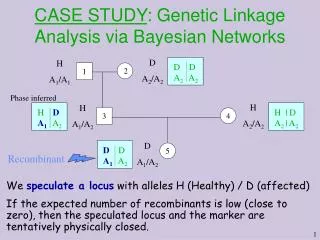
19. ..Continued • Output: the probability of the observed data, given some probability model for the transmission of alleles. Composed of: founder probabilities - Hardy-Weinberg equilibrium penetrance probabilities - The probability of the phenotype, given the genotype transmission probabilities - the probability of a child having a certain genotype given the parents’ genotypes

20. ..Continued • Bottom-Up: sum conditioned probabilities over all possible genotypes of the children and only then on the possible genotypes for the parents. • Linear in the number of people.

21. Lander-Green method • Computes the probability of marker genotypes, given an inheritance vector. P(Mi|Vi) at locus i A certain inheritance vector. marker data at this locus (evidence).

22. Main Idea • Let a = (a1,…,a2f) be a vector of alleles assigned to founders of the pedigree (f is the number of founders). • We want a graph representation of the restrictions imposed by the observed marker genotypes on the vector a that can be assigned to the founder genes. • The algorithm extracts only vectors a compatible with the marker data. • Pr[m|v] is obtained via a sum over all compatible vectors a.

23. 1 2 11 12 13 14 a/b a/b 21 22 23 24 a/b a/b b/d a/c Example – marker data on a pedigree

24. 1 2 11 12 13 14 a/b a/b 21 22 23 24 a/b a/b b/d a/c Example – Descent Graph Descent Graph 3 4 5 6 1 2 7 8 (a,b) (a,b) (a,b) (a,b) (a,c) (b,d)

25. Descent Graph 3 4 5 6 1 2 7 8 (a,b) (a,b) (a,b) (a,b) (a,c) (b,d) • Assume that paternally inherited genes are on the left. • Assume that non-founders are placed in increasing order. • A ‘1’ (‘0’) is used to denote a paternally (maternally) originated gene. •  The gene flow above corresponds to the inheritance vector: v = ( 1,1; 0,0; 1,1; 1,1; 1,1; 0,0 )

26. (a,b) (a,b) (a,c) (b,d) (a,b) Example – Founder Graph Descent Graph 3 4 5 6 1 2 7 8 (a,b) (a,b) (a,b) (a,b) (a,c) (b,d) Founder Graph 5 3 6 4 2 1 8 7

27. (a,b) (a,b) 5 3 6 4 (a,c) (b,d) (a,b) 2 1 8 7 Find compatible allelic assignments for non-singleton components • Identify the set of compatible alleles for each vertex. This is the intersection of the genotypes. {a,b} ∩ {a,b} = {a,b} {a,b} ∩{b,d} = {b}

28. (a,b) (a,b) 5 3 6 4 (a,c) (b,d) (a,b) 2 1 8 7 Possible Allelic Assignments {b} {a} {a,b} {a,b} {a,b,c,d} {a,b} {b,d} {a,c}

29. If for some component there are no possible allelic assignments, then P(m|v) = 0. The probability of singleton components is 1  we can ignore them. Let ahi be an element of a vector of alleles assigned to the vertices of component Ci. Computing P(m|v) over 2f elements 2 terms at most Linear in the number of founders

30. Latest News: SuperLink • Combines the covered approaches in one unified program. • Has other built-in abilities that increase its computations efficiency. • Claimed to be more capable and faster than other related programs (by its own makers). • http://bioinfo.cs.technion.ac.il/superlink/

31. The End