Download

1 / 36
380 likes | 573 Views
Petri nets for Process Planning. What is a Petri net ? Calculating with Petri nets: the reachability graph Petri nets for process planning Optimising routings with Petri nets. Component A. Component B. Assembly A+B C. Component C. What is a Petri net ?. p1. Assembly

E N D
Petri nets for Process Planning Whatis a Petri net ? CalculatingwithPetri nets: the reachability graph Petri nets for process planning OptimisingroutingswithPetri nets
Component A Component B Assembly A+B C Component C What is a Petri net ?
p1 Assembly A+B->C p3 Component A 1 1 Component C 1 Component B t1 p2 State before assembly State after assembly How do we model it with Petri nets ? Model input buffers & more Model manufacturing actions Model output buffers & more Model manufacturing states
Transition Place Arc Arc weight 1 Token Enabling Firing-1 Firing-2 What are the constructing elements of a Petri net ? Input place Output place 2
p1 Component A 1 1 1 Component B p2 Questions : Assembly A+B->C p3 • What happens if there are no tokens in one or both of the two places p1 and p2 ? • What is the meaning of the number of tokens in place p3 ? • Can you see the difference between the two states of the Petri net above, before and after the assembly operation? • Can you, from your observation, derive a definition for the “state” of a Petri net? Component C t1
Petri net definitions A Petri net is a four-tuple: where: Pis a finite non-empty set of n=|P|places Tis a finite non-empty set of m=|T|transitions i.e. places and transitions are disjoint sets is the the pre-incidence or input function is the the post-incidence or output function
Petri net definitions (cont. 1) There is an arc from place pito transition tj iff There is an arc from transition tk to place pi iff { Arc weight:
A simple Petri net P = (p1, p2, p3, p4, p5) p1 p2 p3 T = (t1) I(p1, t1) = 3 I(p2, t1) = 1 I(p3, t1) = 2 3 2 t1 2 p5 p4 O(t1, p4) = 2 O(t1, p5) = 1
p1 p2 p3 3 2 t1 2 p5 p4 Marking M(p) : number of tokens at a placep local state of the place ex. : M(p3) = 2 MarkingM : vector n = |P| (the state vector) pth component of n = M(p) 4 1 2 1 0
Initial marking p1 p2 p3 3 2 t 2 p5 p4 Marked Petri net A Petri net with initial marking i.e. some tokens in some places • N = < P , T , I , O, M0>
7 p4 2 t1 p1 2 1 p2 1 8 p5 1 17 3 p3 16 You make some practice ! • What is the initial markingM0 of the Petri net shown below ? • How many times you may fire transition t1 ? • What is the marking after the final firing (final marking MF)? Note: Numbers in places indicate number of tokens
The token game more formally Enabling rule A transition t is enabled at M iff M I(t) Firing rule
p5 t1 t5 p1 …and its RG M0 p4 t2 1,0,1,0,0 t1 t3 M1 M2 t3 p2 t4 t1 0,0,1,0,1 1,1,0,0,0 p3 t3 t2 M5 M4 A Petri net … t5 t4 M3 0,0,0,0,0 0,0,1,1,0 0,1,0,0,1 t3 t5 M6 0,1,0,1,0 Petri net analysis : the reachability graph
p5 M0 t1 p1 t5 1,0,1,0,0 p4 t2 p5 t1 p2 t4 p1 t3 t5 p3 t3 t1 p4 t2 M2 M1 p5 t1 p1 p2 t4 t5 t3 p3 t1 0,0,1,0,1 1,1,0,0,0 p4 t2 t3 t2 p2 t4 M5 M3 M4 t3 p3 p5 t5 t1 p1 t5 t4 0,1,0,0,1 0,0,1,1,0 0,0,0,0,0 p4 t2 p5 t1 p1 t5 p2 t4 p5 t1 t3 p3 t5 t3 p1 p4 t2 t5 p2 t4 p4 t2 t3 p3 p2 t4 t3 p3 p5 t1 M6 p1 t5 p4 t2 0,1,0,1,0 p2 t4 t3 p3 Petri net analysis : the reachability graph construction in detail
Arad Berlin Lsne Geneva Basel Zürich Dublin London Athens Paris Brussels Breadth-first search • Expand shallowest unexpanded node • Implementation: put successors at end of queue
Breadth-first-search algorithm to compute the RG 1. Init: RG := { } toDoList := {M0} 2. whiletoDoListnot { }do 3. take first element fromtoDoList: m 4. remove m fromtoDoList 5. computetransitionFireList(m) 6. foreachtintransitionFireList(m)do 7. m’ := fire(m,t) 8. ifm’not inRG 9. then 10. enterm’inRG 11. appendm’totoDoList 12. fi 13. enterarc(m,m’)inRG 14. od 15. od
t1 t3 M1 M2 0,0,1,0,1 1,1,0,0,0 Breadth-first-search algorithm to compute the RG M0 1,0,1,0,0 1) toDoList = {M0} RG = {M0} take M0 toDoList = { } transitionFireList(M0) = {t1,t3} fire(M0,t1) = M1 M1 RG toDoList = {M1} RG = {M0,M1} arc(M0,M1) = t1 fire(M0,t3) = M2 M2 RG toDoList = {M1,M2} RG = {M0,M1,M2} arc(M0,M2) = t3
M1 M2 0,0,1,0,1 1,1,0,0,0 t3 t5 M3 M4 0,1,0,0,1 0,0,1,1,0 Breadth-first-search algorithm to compute the RG 2) toDoList = {M1,M2} RG = {M0,M1,M2} M0 1,0,1,0,0 take M1 toDoList = {M2} transitionFireList(M1) = {t3,t5} fire(M1,t3) = M3 M3 RG toDoList = {M2, M3} RG = {M0,M1 ,M2 ,M3} arc(M1,M3) = t3 fire(M1,t5) = M4 M4 RG toDoList = {M2,M3 ,M4} RG = {M0,M1,M2 ,M3 ,M4} arc(M1,M4) = t5 t1 t3
t1 t2 M5 0,0,0,0,0 Breadth-first-search algorithm to compute the RG M0 1,0,1,0,0 3) toDoList = {M2,M3 ,M4} RG = {M0,M1,M2 ,M3 ,M4} t1 t3 take M2 toDoList = {M3 ,M4} transitionFireList(M2) = {t1,t2} fire(M2,t1) = M3 M3 RG toDoList = {M3 ,M4} RG = {M0,M1,M2 ,M3 ,M4} arc(M2,M3) = t1 fire(M2,t2) = M5 M5 RG toDoList = {M3 ,M4 ,M5} RG = {M0,M1,M2 ,M3 ,M4 ,M5} arc(M2,M5) = t2 M2 M1 0,0,1,0,1 1,1,0,0,0 t5 t3 M3 M4 0,1,0,0,1 0,0,1,1,0
t5 M6 0,1,0,1,0 Breadth-first-search algorithm to compute the RG 4) toDoList = {M3 ,M4 ,M5} RG = {M0,M1,M2 ,M3 ,M4 ,M5} M0 1,0,1,0,0 take M3 toDoList = {M4 ,M5} transitionFireList(M3) = {t5} fire(M3,t5) = M6 M6 RG toDoList = {M4 ,M5 ,M6} RG = {M0,M1,M2 ,M3 ,M4 ,M5 ,M6} arc(M3,M6) = t5 t1 t3 M1 M2 0,0,1,0,1 1,1,0,0,0 t1 t5 t3 t2 M3 M4 M5 0,1,0,0,1 0,0,1,1,0 0,0,0,0,0
t4 t3 Breadth-first-search algorithm to compute the RG M0 1,0,1,0,0 5) toDoList = {M4 ,M5 ,M6} RG = {M0,M1,M2 ,M3 ,M4 ,M5 ,M6} t1 t3 take M4 toDoList = {M5 ,M6} transitionFireList(M4) = {t3,t4} fire(M4,t3) = M6 M6 RG toDoList = {M5 ,M6} RG = {M0,M1,M2 ,M3 ,M4 ,M5 ,M6} arc(M4,M6) = t3 fire(M4,t4) = M5 M5 RG toDoList = {M5 ,M6} RG = {M0,M1,M2 ,M3 ,M4 ,M5 ,M6} arc(M4,M5) = t4 M1 M2 0,0,1,0,1 1,1,0,0,0 t1 t5 t3 t2 M3 M4 M5 0,1,0,0,1 0,0,1,1,0 0,0,0,0,0 t5 M6 0,1,0,1,0
Breadth-first-search algorithm to compute the RG M0 6) toDoList = {M5 ,M6} RG = {M0,M1,M2 ,M3 ,M4 ,M5 ,M6} 1,0,1,0,0 t1 t3 take M5 toDoList = {M6} transitionFireList(M3) = { } M1 M2 0,0,1,0,1 1,1,0,0,0 t1 t5 t3 t2 M3 M4 M5 t4 0,1,0,0,1 0,0,1,1,0 0,0,0,0,0 7) toDoList = {M6} RG = {M0,M1,M2 ,M3 ,M4 ,M5 ,M6} t3 t5 take M6 toDoList = { } transitionFireList(M6) = { } M6 0,1,0,1,0
p5 t1 t5 p1 …and its RG M0 p4 t2 1,0,1,0,0 t1 t3 M1 M2 t3 p2 t4 t1 0,0,1,0,1 1,1,0,0,0 p3 t3 t2 M5 M4 A Petri net … t5 t4 M3 0,0,0,0,0 0,0,1,1,0 0,1,0,0,1 t3 t5 M6 0,1,0,1,0 Petri nets recall …
This is a simple example part 2 3 5 4 1 Petri nets for process planning • For simplification, consider only one finishing operation per feature. • And this is its matrix of anteriorities.
2 3 5 p6 4 p9 p7 p8 1 p1 p2 p3 p4 p5 p0 Let’s construct the process planning Petri net • Operations • Anteriorities • Each operation only once • One operation at a time 1F 5F 4F 2F 3F
Constraint Places Transitions (manufacturing operations) Input Places (with one initial token) ControlPlace (with one initial token) Formal definition of the process planning Petri net CP1 CP4 CP2 CP3 T1 T5 T4 T2 T3 IP1 IP3 IP5 IP2 IP4 N =[P, T, F, M0, MF]
p6 2 p8 p7 M0 1,1,1,1,1,1,0,0,0,0 3 M1 1F 1F 5F 4F 2F 3F 5 1,0,1,1,1,1,1,1,0,0 p4 p3 M3 M2 4F 2F 4 p9 p5 1 1,0,1,1,0,1,0,1,0,1 1,0,0,1,1,1,1,0,1,0 p0 5F 3F 2F 4F M6 M4 M5 1,0,1,1,0,0,0,1,0,0 1,0,0,1,0,1,0,0,1,1 1,0,0,0,1,1,1,0,0,1 p1 p2 5F 3F 4F 2F M7 M8 1,0,0,1,0,0,0,0,0,0 1,0,0,0,0,1,0,0,0,1 3F 5F MF 1,0,0,0,0,0,0,0,0,0 Process planning RG • Reachability Graph!
1F 2F 3F 4F 5F A process plan in the RG M0 1,1,1,1,1,1,0,0,0,0 M1 1F 1,0,1,1,1,1,1,1,0,0 4F M2 2F M3 1,0,1,1,0,1,0,1,0,1 1,0,0,1,1,1,1,0,1,0 5F 3F 2F 4F M4 M6 M5 1,0,1,1,0,0,0,1,0,0 1,0,0,1,0,1,0,0,1,1 1,0,0,0,1,1,1,0,0,1 5F 3F 4F 2F M7 M8 1,0,0,1,0,0,0,0,0,0 1,0,0,0,0,1,0,0,0,1 3F 5F MF 1,0,0,0,0,0,0,0,0,0
How to consider alternative routings in production planning ? • The Petri net model • establishes a network of possible routings • defers to a later stage the decision of which path to take • the choice of path may be changed after each operation • Alternative routings… • as a function of available resources (machinery, tooling, etc.) • are available in the Petri net model
2 3 5 p6 4 p9 p7 p8 1 5F 2F1 2F2 4F 3F 1F p1 p2 p3 p4 p5 p0 Process planning Petri net with alternatives Assume that operation 2F may be realized in a different alternative machine O1 = [1F, M1(S11, T11)] O21 = [2F1, M1(S11, T12)] O22 = [2F2, M2(S21, T21)] O3 = [3F, M2(S21, T21)] O4 = [4F, M1(S11, T12)] O5 = [5F, M2(S22, T22)]
RG with alternatives O1 O1 O22 O22 O21 O4 O3 O4 O3 O3 O21 O22 O4 O5 O5 O3 O4 O3 O21 O22 O4 O5 O3 O5 O3 O3 O5 O5
How to chose the best process plan among all included in the RG ? • Four types of cost: • (i) the pure machining cost, • (ii) the cost of moving a part from one machine to another, • (iii) the cost of a setup change in one machine and • (iv) the cost of a tool change in one machine. Optimisation criterion : manufacturing cost !
Recall the manufacturing heuristics ! • Keep the same machine as long as possible • quality • economy • Keep the same setup as long as possible • quality • economy • Keep the same tool as long as possible • economy
2 3 5 4 1 Calculating optimal process plans O1 = [1F, M1(S11, T11)] O21 = [2F1, M1(S11, T12)] O22 = [2F2, M2(S21, T21)] O3 = [3F, M2(S21, T21)] O4 = [4F, M1(S11, T12)] O5 = [5F, M2(S22, T22)] opCost [1] = 60 opCost [21] = 50 opCost [22] = 20 opCost [3] = 30 opCost [4] = 50 opCost [5] = 35 Machine_change_cost: = 600 Setup_change_cost:= 400 Tool_change_cost:= 100
2 3 5 4 1 The optimal solution operation machine setup tool opCost totalCost O1 M1 S11 T11 60 1160 O4 M1 S11 T12 50 2280 O22 M2 S21 T21 20 2430 O3 M2 S21 T21 30 2460 O5 M2 S22 T22 35 2995 O1 – O4 – O22 – O3 – O5
Source node O1 O4 O22 O21 O4 O3 O22 O3 O21 O4 O5 O3 O5 O4 O3 O21 O22 O5 O5 O3 O5 O3 O3 Final node PROBLEM ? O1 – O4 – O22 – O3 – O5 How to find the optimal solution in such a graph ? In other words … How to find the shortest path from the « Source node » to the « Final node » ?