Download
1 / 45
450 likes | 681 Views
Introduction to Thermochemistry. In this section we will cover: . Thermochemistry basics (enthalpies, heat of formation, Gibbs free energy) Products of combustion and calculation of flame temperature Numerical methods for equilibrium combustion. Objectives.

E N D
In this section we will cover: • Thermochemistry basics (enthalpies, heat of formation, Gibbs free energy) • Products of combustion and calculation of flame temperature • Numerical methods for equilibrium combustion
Objectives • Understand reaction of propellants. • Calculate combustion chamber gas properties such as the specific heats, molecular weight, and stagnation temperature. Basic difficulty The equilibrium constant of each reaction step depends on temperature. The temperature, in turn, depends on the heat released by reaction, and the molecular weight of the mixture (i.e., the composition). Thus we must solve for the composition and temperature simultaneously.
Two further complications arise: The exothermic reactions which characterize combustion of rocket propellants, conform to the Arrhenius Reaction Rate Expression where r is the reaction rate (i.e., mass of reactants produced per unit time) , T is temperature, A is either constant or a weak function of temperature, and E and R are respectively, the “activation energy” and the mixture gas constant. In addition, combustion reactions proceed very quickly, once a temperature threshold is exceeded. To calculate the composition accurately, a set of differential equations must be solved, with vastly different rates. This again challenges numerical algorithms for solving differential equations.
Steps in a typical calculation 1. Guess a Flame Temperature T0 (temperature at which most of the reaction occurs). 2.Determine the equilibrium composition at this temperature, using tabulated equilibrium constants or by minimizing the Gibbs Free Energy. 3.Compare the heat required to raise the products to this temperature with the available heat release according to the composition. 4.Iterate on the guessed temperature until these heats match. 5.Obtain the gas mixture properties at this temperature.
Basics The (g) denotes gas phase. In the above, the reaction goes both ways. In a mixture of hydrogen, oxygen and water vapor, the concentration of water vapor increases if the temperature increases, since the “forward reaction rate” increases with temperature, much more than the “backward reaction rate” increases, and the equilbrium constant shifts to the right.
Heat of reaction: constant-pressure process If hydrogen and oxygen are present in the proportion indicated above, the mixture is said to be “stoichiometric”. For a constant-pressure process (typical rocket engine process) it is convenient to write the heat Q as the change in total enthalpy. Thus, Q = -H The reactions involved in a typical rocket engine process can be exothermic (heat is released as the reaction proceeds in the forward direction) or endothermic (heat is absorbed in the forward direction). “Heat of Reaction” DH = H products - H reactants
For exothermic reactions, DH <0 It is often convenient to write the energy available in a molecule as Heat of Formation = DHf0 = DQf0 where the 0 superscript indicates standard conditions: temperature of 298K and pressure of 1 atm. The heat of formation is the DH to form 1 mole of the substance from its constituent elements. By convention, the most stable constituent elements are assumed to have DHf0 of zero. (example: Nitrogen, N2 ) For example, assuming that the reaction exists at STP (standard temperature, 300K, and pressure, 1 atm), let’s consider 1 molecule of gaseous diatomic hydrogen reacting with 1 mole of diatomic oxygen gas to form 1 mole of liquid hydrogen peroxide. The enthalpy of 1 mole of hydrogen peroxide is less than that of the reactants by 187.67 KiloJoules. Thus, for this reaction, DHf0= -187.67 KJ/mole for liquid hydrogen peroxide.
Knowing the standard heats of formation of several common molecules, we can later estimate the heat of reaction. Examples H2O(g) = -241.93 KJ/mole CO2(g) = -393 KJ/mole O2(g) = 0 H2(g) = 0 N2H4(l) = 50.48 KJ/mole In general, we want the reactants to have a very high, positive DHf0 and the products to have a low DHf0
Compound KJ/mol Compound KJ/mol Al(s) 0 N2(g) 0 Al2O3 -1670.53 N(g) +472.71 C(s, graphite) 0 NH3(l) -65.63 CO(g) -110.59 NH3(g) -46.21 CO2(g) -393.68 N2H4(l) +50.48 C(g) +718.70 N2O4(l) -20.13 CH4(g) -74.90 NH4CLO4(s) -290.58 CH3OH(l) -238.76 HF(g) -268.73 C2H5OH(l) -277.77 HC(g) -92.34 H2(g) 0 F2(l, 85k) -12.68 H2(l, 20K) -7.03 O2(g) 0 H(g) +218.04 O2(l, 90K) -9.42 H2O(g) -241.93 H2O(l) -285.96 H2O2(l) -187.69 HNO3(l) -173.08 Note: Since heat is released when the standard heat of formation is less than 0, many books will use Qf0 = -DHf0 as the heat of formation. Here Qf0 is the heat released for isothermal reaction. Most heat of formation values are determined experimentally. However, for reactions which do not normally occur at STP, we can use Hess’ Law which allows two reactions to be added algebraically to estimate a third.
Hess’ Law Example C + O2 CO2(g) -393.68 KJ/mole CO + ½ O2 CO2(g) -283.09 KJ/mole Adding, C + ½ O2 CO -110.59 KJ/mole Note: 1Kcal = 4.190 KJ
Heat of reaction for a general reaction at STP General Reaction where i denotes each of the reactants. Example at STP (all gases) H2 + CO2 H2O + CO + Qr0 DHrxn0 = { 1(-241.93) + 1(-110.59)} – {1(0) + 1(-393.68)} = 41.16 KJ So Qr0 = - 41.16 kJ endothermic.
Reactions occurring at temperatures other than STP Since enthalpy is a state function of temperature (for a thermally perfect gas) the path to a certain composition and temperature is not important. At a higher temperature, Note that Cp = Cp(T) can be obtained from a curve fit. Note also that any phase changes must be accounted. H2O(s) H2O(l) + 6.00 kJ/mole at 273K. H2O(l) H2O(g) +40.7 kJ/mole at 373K
The Available Heat Method – Flame Temperature Temporarily, let us ignore the effect of temperature and pressure on the equilibrium composition and assume that we have a reaction that proceeds to completion left to right (as would be the case at high pressure or low flame temperatures, per Le Chatelier’s principle. At 200 atm, with a fuel-rich mixture 5H2 + 1O2 2H2O + 3H2 Assume that all species are gases and that the products enter the chamber at 500K = Ti.
We will view the heat release process as a hypothetical 3-step process, because the data on heats of formation are usually tabulated at STP (Standard Temperature and Pressure): 1.All the constituents of the mixture are cooled down to the standard heat of formation at STP (298K and 1 atm). 2.Reaction proceeds in an isothermic manner (temperature does not change). 3.Once the total heat available is calculated, the final temperature reached is calculated. Once the products are created at STP, the available heat is used to raise the temperature to Tf. This is the Required Heat.
Example given in Humble p. 170 The process requires us to iterate to determine Tc – easier if the n’s don’t change, in which case Q available is constant. Returning to our hydrogen-oxygen example: 5H2 + 1O2 2H2O + 3H2 (Heat released when the more stable water-molecule bonds are created.) Heat at initial conditions: O2 @ 500K = 6.057 KJ/mole H2 @ 500K = 5.831 KJ/mole
Find Tc Guess Tc = 2800K From Tables From Tables Too low. Increase guess of Tc to 3000K Close, but high. Linear interpolation should be OK as a guess over a small range: Tc=2998K
Calculating mixture properties at the final temperature Mixture molecular weight: where Recall: To get Cpi’ we either use Tables or calculate directly from equations. Example (units are BTU/(lbm-moleR); T in deg.R; in the range 540 < T <5400; ) For H2O.
Equilibrium Analysis Our previous calculations assumed that the final composition was known – and essentially assumed that the reaction proceeded in only the forward direction. Now we consider how to deal with the realistic situation where the composition changes with temperature. A simple reaction may be described as where a,b,c,d are called the “stoichiometric coefficients. The rates kf and kb denote rates of the forward and backward reaction steps respectively. The state of Chemical Equilibrium is defined as one where the concentrations do not change with time. If the external state variables do not change with time. Thus, for a given pressure and temperature, there is a unique combination of the stoichiometric coefficients a,b,c and d.
Some Features of Chemical Equilibrium • Concentrations at equilibrium depend only on state properties (pressure and temperature). • In terms of Statistical Mechanics, the state of equilibrium involves a much larger number of “microstates” than other states – in other words, most of the time, a system can be found at or very near the equlibrium state. • Relaxation towards equilibrium from a disturbed state generally involves increase in entropy (this is • used in the “Gibbs Free Energy” method to calculate equilibrium properties.
Equilibrium Constants Define Pa = partial pressure of species “a” in equilibrium divided by 1 atm pressure to make dimensionless na = number of moles of species “a” for a mixture of perfect gases For a generic equilibrium reaction The equilibrium constant in terms of partial pressures is
These Kp’s are tabulated as functions of temperature. There is also a pressure dependence, but it far weaker than the temperature dependence. On the other hand, pressure may change by orders of magnitude between different types of combustors. Kp’s can in principle be computed from “first principles” using quantum mechanics and statistical mechanics, considering probabilities of collisions with the “correct” relative energies and orientations. However, this process has large uncertainties. The tables of equilibrium constants are obtained “empirically” with the interpolation (and some extrapolation) done using the forms derived from first principles, and experimental fits to data.
Equilibrium Constant in Molar Terms Since we ultimately need to determine the number of moles in the products, we need an expression of the equilibrium constant in molar terms We can use this constant along with mass balance for each type of atom to solve for the species in equilibrium.
Example At 10 atm and 4000K , with the initial concentrations at low temperature being ½ mole of H2 and none of H. At equilibrium at 4000K, we have Atom conservation: the only kinds of atoms here are H atoms Thus the above can be re-written as
From Tables Also from the definition
Solving the resulting quadratic equation, we get Take the negative-sign, because we can’t have more than 0.5 moles of H2. This gives: Thus at equilibrium at 4000K, 10 atm, we have
More general example: Lets say that at low temperature we have essentially just diatomic hydrogen and oxygen, in stoichiometric proportions. At equilibrium at the high temperature, we have six unknown concentrations. Need six independent equations. Two of these are easily decided: • Conservation of H atoms • Conservation of O atoms.
The remaining 4 are given by the equilibrium constant for 4 reactions which we select “judiciously” (based on vast prior experience – this in practice, for most overall reactions, is a matter of some uncertainty, as we have to decide which substances are likely to be present with significant concentrations at equilibrium. This last decision also involves some consideration of our objectives – whether the objective is to calculate performance of the system, which requires good accuracy in heat release and eventual temperature and exhaust gas molecular weight, or the presence of pollutants, which may only be present in trace quantities. Here we select Kp for
Gibbs Free Energy Method A second method for determining equilibrium is the minimization of Gibbs Free Energy G. Note that this method is closely related to the equilibrium constant method. Gibbs Free Energy is a function of temperature and pressure (the latter through S).For a given species (1 atm – although for an ideal gas this doesn’t matter) – Gibbs Free Energy of Formation (available in tables) – Function of temperature partial pressure referenced to 1 atm. Note Universal Gas Constant for use of these tables
=number of moles of “i” at equilibrium So, for each species in the combustion products For the mixture then, all species cal or J At a given stagnation pressure and temperature, the composition will be in equilibrium when G is minimized. Note that we must still conserve the number of each atom (O, H, etc) – 1 constraint per atom type. For our previous example, stagnation pressure is 10 atm and stagnation temperature is 4000K.
Before the combustion reaction occurs, we have ½ mole of H2 and none of H. When the combustion reaction reaches equilibrium at the final temperature these change to and respectively Atom conservation of By Gibbs Free Energy method
For minimum , In general, this method can be complex . The number of moles of each species is iterated to drive G to its minimum while maintaining conservation of each atom in the mix. Computer programs are able to determine this solution relatively quickly for a given P and T (Gordon and McBride, CEA code). Examples 1.CEA 2.STANJAN 3.GasEQ
Relationship Between Equilibrium Constants and Gibbs Ultimately, these two methods are related. It can be shown Where: For our reaction at 4000K =1.5933
Check The Gibbs Free Energy Method is more common for computer applications.
Equilibrium Constants Define Pa = partial pressure of species “a” in equilibrium divided by 1 atm pressure to make dimensionless na = number of moles of species “a” for a mixture of perfect gases For a generic equilibrium reaction The equilibrium constant in terms of partial pressures is
Same problem with a different choice of reactions Consider a mixture which is essentially all diatomic hydrogen and oxygen at low temperatures. When the reaction proceeds to a high final temperature, we have a mixture with unknown concentrations of several substances. Atom conservation: Results from STANJAN 4000K; 10 ATM; case of a=2, b=1 Reaction scheme is:
Effect of Mixture Ratio on Isp Ref: Hill & Peterson, p. 573 • Peak Isp (>460sec)predicted to occur at stoichiometric mixture ratio – if dissociation products are ignored. • Peak stagnation temperature occurs at stoichiometric • Due to dissociation, Isp drops steeply at the higher temperatures. • Actual Peak Isp (~ 410 sec.) occurs at an oxidizer-fuel ratio which is roughly half the stoichiometric!
Effect of Pressure on Isp Increased pressure is good to reduce dissociation at the higher temperatures – enables higher Isp. Remember that higher chamber pressure is also good because it increases the thermodynamic cycle efficiency. - Higher exhaust velocity.
Characteristic Exhaust Velocity c* Used to characterize the performance of propellants and combustion chambers independent of the nozzle characteristics. where is the quantity in brackets. Note: So Characteristic exhaust velocity Assuming steady, quasi-1-dimensional, perfect gas. The condition for maximum thrust is ideal expansion: nozzle exit static pressure being equal to the outside pressure. In other words,
Characteristic Velocity c* As we saw before, the characteristic velocity is calculated based on combustor conditions and a choked nozzle throat.
Review • Types of rocket engines • The rocket equation, and a simple solution process for a launch to orbit. • Single-stage rocket: height reached. • Multi-staging • Calculation of rocket thrust via momentum equation • Definition of Isp, • Mass Ratio for given delta-v. • Thrust coefficient CF, • Characteristic Velocity c*
Review • Orbital mechanics considerations related to mission requirements. Kepler’s laws, Newton’s law of gravitation • Expressions for simple orbits • Hohman transfers. • One-tangent burns • Spiral transfers, continuous-thrust maneuvers. • Orbit Plane Changes • Launch from Earth to GEO: gravity turn, tangent steering
Review • Introduction to thermochemistry: • Heats of formation • Heats of reaction • Equilibrium constants • Calculation of temperature and equilibrium composition in a combustion reaction • Available Heat Method • Gibbs Free Energy method • Relation between Equlibrium constants and Gibbs method • Choosing reaction schemes • Effect of pressure on Isp • Effects of mixture ratio on Isp