Download
1 / 180
1.8k likes | 1.82k Views
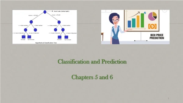
Chapter 5 . Classification and Prediction. What is classification? What is prediction? Issues regarding classification and prediction Classification by decision tree induction Bayesian Classification Classification by Back Propagation Support Vector Machines

E N D
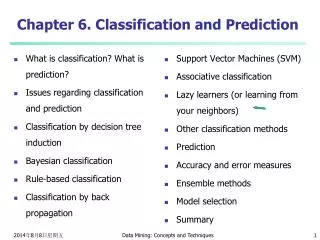
Chapter 5. Classification and Prediction • What is classification? What is prediction? • Issues regarding classification and prediction • Classification by decision tree induction • Bayesian Classification • Classification by Back Propagation • Support Vector Machines • Associative Classification: Classification by association rule analysis • Lazy Learners (or Learning from your Neighbors) • Other Classification Methods • Prediction • Accuracy • Summary Data Mining: Concepts and Techniques
Simple Linear Regression • Simple Linear Regression Model • Least Squares Method • Coefficient of Determination • Model Assumptions • Testing for Significance • Using the Estimated Regression Equation for Estimation and Prediction • Computer Solution • Residual Analysis: Validating Model Assumptions • Residual Analysis: Outliers and Influential Observations Data Mining: Concepts and Techniques
What Is Prediction? • Prediction is similar to classification • First, construct a model • Second, use model to predict unknown value • Major method for prediction is regression • Linear and multiple regression • Non-linear regression • Prediction is different from classification • Classification refers to predict categorical class label • Prediction models continuous-valued functions Data Mining: Concepts and Techniques
Predictive Modeling in Databases • Predictive modeling: Predict data values or construct generalized linear models based on the database data. • One can only predict value ranges or category distributions • Method outline: • Minimal generalization • Attribute relevance analysis • Generalized linear model construction • Prediction • Determine the major factors which influence the prediction • Data relevance analysis: uncertainty measurement, entropy analysis, expert judgement, etc. • Multi-level prediction: drill-down and roll-up analysis Data Mining: Concepts and Techniques
Regress Analysis and Log-Linear Models in Prediction • Linear regression: Y = 0 + 1 X • Two parameters , 0 and 1 specify the line and are to be estimated by using the data at hand. • using the least squares criterion to the known values of Y1, Y2, …, X1, X2, …. • Multiple regression: Y = b0 + b1 X1 + b2 X2. • Many nonlinear functions can be transformed into the above. • Log-linear models: • The multi-way table of joint probabilities is approximated by a product of lower-order tables. • Probability: p(a, b, c, d) = ab acad bcd Data Mining: Concepts and Techniques
The Simple Linear Regression Model • Simple Linear Regression Model y = 0 + 1x+ • Simple Linear Regression Equation E(y) = 0 + 1x • Estimated Simple Linear Regression Equation y = b0 + b1x ^ Data Mining: Concepts and Techniques
Simple Linear Regression Model The population regression model: Random Error term Population SlopeCoefficient Population Y intercept Independent Variable Dependent Variable Linear component Random Error component Data Mining: Concepts and Techniques
Simple Linear Regression Model (continued) Y Observed Value of Y for Xi εi Slope = β1 Predicted Value of Y for Xi Random Error for this Xi value Intercept = β0 X Xi Data Mining: Concepts and Techniques
Simple Linear Regression Equation The simple linear regression equation provides an estimate of the population regression line Estimated (or predicted) y value for observation i Estimate of the regression intercept Estimate of the regression slope Value of x for observation i The individual random error terms ei have a mean of zero Data Mining: Concepts and Techniques
Least Squares Estimators • b0 and b1 are obtained by finding the values of b0 and b1 that minimize the sum of the squared differences between y and : Differential calculus is used to obtain the coefficient estimators b0 and b1 that minimize SSE Data Mining: Concepts and Techniques
Least Squares Estimators (continued) • The slope coefficient estimator is • And the constant or y-intercept is • The regression line always goes through the mean x, y Data Mining: Concepts and Techniques
Finding the Least Squares Equation • The coefficients b0 and b1 , and other regression results in this chapter, will be found using a computer • Hand calculations are tedious • Statistical routines are built into Excel • Other statistical analysis software can be used Data Mining: Concepts and Techniques
Model Assumptions • Assumptions About the Error Term • The error is a random variable with mean of zero. • The variance of , denoted by 2, is the same for all values of the independent variable. • The values of are independent. • The error is a normally distributed random variable. Data Mining: Concepts and Techniques
Linear Regression Model Assumptions • The true relationship form is linear (Y is a linear function of X, plus random error) • The error terms, εi are independent of the x values • The error terms are random variables with mean 0 and constant variance, σ2 (the constant variance property is called homoscedasticity) • The random error terms, εi, are not correlated with one another, so that Data Mining: Concepts and Techniques
Interpretation of the Slope and the Intercept • b0 is the estimated average value of y when the value of x is zero (if x = 0 is in the range of observed x values) • b1 is the estimated change in the average value of y as a result of a one-unit change in x Data Mining: Concepts and Techniques
Simple Linear Regression Example • A real estate agent wishes to examine the relationship between the selling price of a home and its size (measured in square feet) • A random sample of 10 houses is selected • Dependent variable (Y) = house price in $1000s • Independent variable (X) = square feet Data Mining: Concepts and Techniques
Sample Data for House Price Model Data Mining: Concepts and Techniques
Graphical Presentation • House price model: scatter plot Data Mining: Concepts and Techniques
Regression Using Excel • Tools / Data Analysis / Regression Data Mining: Concepts and Techniques
Excel Output The regression equation is: Data Mining: Concepts and Techniques
Graphical Presentation • House price model: scatter plot and regression line Slope = 0.10977 Intercept = 98.248 Data Mining: Concepts and Techniques
Interpretation of the Intercept, b0 • b0 is the estimated average value of Y when the value of X is zero (if X = 0 is in the range of observed X values) • Here, no houses had 0 square feet, so b0 = 98.24833 just indicates that, for houses within the range of sizes observed, $98,248.33 is the portion of the house price not explained by square feet Data Mining: Concepts and Techniques
Interpretation of the Slope Coefficient, b1 • b1 measures the estimated change in the average value of Y as a result of a one-unit change in X • Here, b1 = .10977 tells us that the average value of a house increases by .10977($1000) = $109.77, on average, for each additional one square foot of size Data Mining: Concepts and Techniques
Example: Reed Auto Sales • Simple Linear Regression Reed Auto periodically has a special week-long sale. As part of the advertising campaign Reed runs one or more television commercials during the weekend preceding the sale. Data from a sample of 5 previous sales are shown below. Number of TV AdsNumber of Cars Sold 1 14 3 24 2 18 1 17 3 27 Data Mining: Concepts and Techniques
Example: Reed Auto Sales • Slope for the Estimated Regression Equation b1 = 220 - (10)(100)/5 = 5 24 - (10)2/5 • y-Intercept for the Estimated Regression Equation b0 = 20 - 5(2) = 10 • Estimated Regression Equation y = 10 + 5x ^ Data Mining: Concepts and Techniques
Example: Reed Auto Sales • Scatter Diagram Data Mining: Concepts and Techniques
Measures of Variation • Total variation is made up of two parts: Total Sum of Squares Regression Sum of Squares Error Sum of Squares where: = Average value of the dependent variable yi = Observed values of the dependent variable i = Predicted value of y for the given xi value Data Mining: Concepts and Techniques
Measures of Variation (continued) • SST = total sum of squares • Measures the variation of the yi values around their mean, y • SSR = regression sum of squares • Explained variation attributable to the linear relationship between x and y • SSE = error sum of squares • Variation attributable to factors other than the linear relationship between x and y Data Mining: Concepts and Techniques
Measures of Variation (continued) Y yi y SSE= (yi-yi )2 _ SST=(yi-y)2 _ y _ SSR = (yi -y)2 _ y y X xi Data Mining: Concepts and Techniques
Coefficient of Determination, R2 • The coefficient of determination is the portion of the total variation in the dependent variable that is explained by variation in the independent variable • The coefficient of determination is also called R-squared and is denoted as R2 note: Data Mining: Concepts and Techniques
Examples of Approximate r2 Values Y r2 = 1 Perfect linear relationship between X and Y: 100% of the variation in Y is explained by variation in X X r2 = 1 Y X r2 = 1 Data Mining: Concepts and Techniques
Examples of Approximate r2 Values Y 0 < r2 < 1 Weaker linear relationships between X and Y: Some but not all of the variation in Y is explained by variation in X X Y X Data Mining: Concepts and Techniques
Examples of Approximate r2 Values r2 = 0 Y No linear relationship between X and Y: The value of Y does not depend on X. (None of the variation in Y is explained by variation in X) X r2 = 0 Data Mining: Concepts and Techniques
Excel Output 58.08% of the variation in house prices is explained by variation in square feet Data Mining: Concepts and Techniques
Correlation and R2 • The coefficient of determination, R2, for a simple regression is equal to the simple correlation squared Data Mining: Concepts and Techniques
The Correlation Coefficient • Sample Correlation Coefficient where: b1 = the slope of the estimated regression equation Data Mining: Concepts and Techniques
Example: Reed Auto Sales • Sample Correlation Coefficient The sign of b1 in the equation is “+”. rxy = +.9366 Data Mining: Concepts and Techniques
Estimation of Model Error Variance • An estimator for the variance of the population model error is • Division by n – 2 instead of n – 1 is because the simple regression model uses two estimated parameters, b0 and b1, instead of one is called the standard error of the estimate Data Mining: Concepts and Techniques
Excel Output Data Mining: Concepts and Techniques
Comparing Standard Errors se is a measure of the variation of observed y values from the regression line Y Y X X The magnitude of se should always be judged relative to the size of the y values in the sample data i.e., se = $41.33K ismoderately small relative to house prices in the $200 - $300K range Data Mining: Concepts and Techniques
Inferences About the Regression Model • The variance of the regression slope coefficient (b1) is estimated by where: = Estimate of the standard error of the least squares slope = Standard error of the estimate Data Mining: Concepts and Techniques
Excel Output Data Mining: Concepts and Techniques
Comparing Standard Errors of the Slope is a measure of the variation in the slope of regression lines from different possible samples Y Y X X Data Mining: Concepts and Techniques
Inference about the Slope: t Test • t test for a population slope • Is there a linear relationship between X and Y? • Null and alternative hypotheses H0: β1 = 0 (no linear relationship) H1: β1 0 (linear relationship does exist) • Test statistic where: b1 = regression slope coefficient β1 = hypothesized slope sb1 = standard error of the slope Data Mining: Concepts and Techniques
Inference about the Slope: t Test (continued) Estimated Regression Equation: The slope of this model is 0.1098 Does square footage of the house affect its sales price? Data Mining: Concepts and Techniques
H0: β1 = 0 H1: β1 0 Inferences about the Slope: tTest Example b1 From Excel output: t Data Mining: Concepts and Techniques
H0: β1 = 0 H1: β1 0 Inferences about the Slope: tTest Example (continued) Test Statistic: t = 3.329 b1 t From Excel output: d.f. = 10-2 = 8 t8,.025 = 2.3060 Decision: Conclusion: Reject H0 a/2=.025 a/2=.025 There is sufficient evidence that square footage affects house price Reject H0 Do not reject H0 Reject H0 tn-2,α/2 -tn-2,α/2 0 -2.3060 2.3060 3.329 Data Mining: Concepts and Techniques
H0: β1 = 0 H1: β1 0 Inferences about the Slope: tTest Example (continued) P-value = 0.01039 P-value From Excel output: This is a two-tail test, so the p-value is P(t > 3.329)+P(t < -3.329) = 0.01039 (for 8 d.f.) Decision: P-value < α so Conclusion: Reject H0 There is sufficient evidence that square footage affects house price Data Mining: Concepts and Techniques
Confidence Interval Estimate for the Slope Confidence Interval Estimate of the Slope: d.f. = n - 2 Excel Printout for House Prices: At 95% level of confidence, the confidence interval for the slope is (0.0337, 0.1858) Data Mining: Concepts and Techniques
Confidence Interval Estimate for the Slope (continued) Since the units of the house price variable is $1000s, we are 95% confident that the average impact on sales price is between $33.70 and $185.80 per square foot of house size This 95% confidence interval does not include 0. Conclusion: There is a significant relationship between house price and square feet at the .05 level of significance Data Mining: Concepts and Techniques