Download
1 / 30
310 likes | 410 Views
,. STATISTICAL DATA ANALYSIS Carlos Artur S. Rocha, Ph.D. DESCRIPTIVE STATISTICS Frequency Distributions

E N D
, STATISTICAL DATA ANALYSIS • Carlos Artur S. Rocha, Ph.D.
DESCRIPTIVE STATISTICS Frequency Distributions • When colleting and summarizing large amount of data, it is often helpful to record the data in the form of a frequency table. Such a table simply involves a listing of all the observed values of the variable being studied and how many times each value is observed. • Consider, for instance, the tabulation of the frequency of occurrence of benthic sea weed in New World mangrove, Table 1.
Table 1 – Illustration of the distribution of benthic sea weed in New World mangrove.
One can also make a frequency distribution by grouping the data into size classes. Such grouping results in the loss of some information and is generally utilized only to make frequency tables and bar graphs easier to read. • There have been several “rules of thumb” proposed to aid in deciding into how many classes data might reasonably be grouped. • A useful series of steps for forming a frequency distribution is given below . These steps are applied to the following data set:
33 – 35 – 35 – 39 – 41 – 41 – 42 – 45 – 47 – 48 – 50 – 52 – 53 – 54 – 55 55 – 57 – 59 – 60 – 60 – 61 – 64 – 65 – 65 – 65 – 66 – 66 – 66 – 67 – 68 69 – 71 – 73 - 73 – 74 – 74 – 76 – 77 – 77 – 78 – 80 – 81 – 84 – 85 – 85 88 – 89 – 91 – 94 – 97 1- Determine the range of the ungrouped numbers: R = 97 – 33 = 64 2- Select the number of classes (k) into which the range will be divided. As a rule of thumb, the number of classes should be between 5 and 20. k = 1 + 3,22 log N = 1 + 3,22x1,7 = 7
3 – Divide the number of classes into the range and round the result to the next largest integer. This number represents de class width (h) of each class. h = R/k = 64/7 = 10 4- Select the class limits by beginning with the smallest number and constructing classes with the width determined in step 3.
In presenting this frequency distribution graphically, one can prepare a histogram, which is the name given to a bar graph based on continuous data.
MEASURES OF CENTRAL TENDENCY • Various measures of central tendency are useful parameters, in that they describe a property of populations. We will discuss the characteristics of these parameters and the sample statistics that are good estimates of them.
The most widely used measure of central tendency is the arithmetic mean, which is the measure most commonly called an average. The Arithmetic Mean • The calculation o the population mean can be abbreviated concisely by the formula: 𝛍 = Where the size of the population (which we generally do not Know) is denoted as N.
The most efficient, unbiased, and consistent estimate of the population mean 𝛍, is thesamplemean, denoted as Xbar (read “Xbar”) is calculated as Xbar =
PropertyofArithmeticMean 1- The algebric sum of the deviation of a set of value from the mean is zero. That is: 2- The algebric sum of the square of the deviations of a set of value from the mean is minimum. That is:
If, as in example of determination of the amount of phosphorus in leaves, Xi can be said to denote each of k different measurements and fi can denote the frequency with which that Xi occurs in the sample. The sample mean may then be calculated as
The Mode The mode is commonly defined as the most frequently occurring measurement in a set of data. For some frequency distributions may have more than one such point of concentration, even though these concentrations might not contain the same frequencies.
The Median The median is typically defied as the middle measurement in an ordered set of data. That is, there are just as many observations larger than the median as there are samller. The median (M) of a sample of data may be found by first arranging the measurements in ascending or descending order of magnitude.
Then, we define the sample median as M = X(n + 1)/2 If the sample size (n) is odd, then the subscript will be an integer and will indicate which datum is the middle measurement. If n is even, then the subscript will be a half-integer, a number midway between two integers. The median is defined as the midpoint between them.
Measures of Dispersion and Variability In addition to a measure of central tendency, it is desirable to have a measure of dispersion or a measure of variabiliyof data. It is an indication of the spread of measurements around the center of the distribution.
The Population Variance Denoted as δ2 thepopulationvariance, It is defined as: δ2 =
The Sample Variance Thebestestimateofthepopulationvarianceδ2 , is the samplevariance - S2 is defined as: S2 =
The Standard Deviation It is the square root of the variance. Therefore, it has the same units as the original measurements. Thus, for a population, δ= √ δ2 And for a sample, S= √ S2
The Coefficiente of Variation The coefficient of variation is defined as: CV = (S/ Xbar) x 100 % Since S and Xbar have identical units, CV has no units at all, a fact emphasizing that it is a relative measure, divorced from the actual magnitude or units of measurement of the data. Thus, had the data been measured in pound, kilograms or grams, the calculated CV would have the same.
The Normal Distribution The basic form of the normal distribution is that of a bell – it has a single mode and is symmetric about its central value.
A continuous random variable X is said to be normally distributed if its probability density function is: f(x) = where 𝛍andδ are parameters of the distribution and Π (pi), ande (the base ofNaperian, or natural logarithms) are mathematicalconstantequal to 3.14159... and 2.71828...respectively.
Recall that the probability of a continuous variable assuming a value between a and b P(a <= X <= b) can be determined by finding the area under its density function from a to b. As we shall see, it is possible to determine the area by using the standard normal distribution
A normal distribution with 𝛍 = 0 and = 1 is called a standard normal distribution. When a normal variable X has a mean zero and a variance 1, de variable will be denoted by Z: Z = (X - 𝛍)/
Uma outra forma de avaliarmos a magnitude de evidência contra Ho é pelo valor-p do teste, definido como a probabilidade de se obter, em outra amostra, um valor mais extremo para a estatística do que o obtido pela amostra considerada, dado que Ho é verdadeira. • No teste da média o valor-p é expresso como:
The most widely used measure of central tendency is the arithmetic mean. The Arithmetic Mean Let Xi be the measurement of Xi , X2 ,…, Xn