Download
1 / 16
180 likes | 446 Views
FFT Convolution. Michael Phipps Vallary S. Bhopatkar. Convolution theorem. Convolution theorem for continuous case: h(t) and g(t) are two functions and H(f) and G(f) are their corresponding Fourier Transform, then convolution is defined as

E N D
FFT Convolution Michael Phipps Vallary S. Bhopatkar
Convolution theorem • Convolution theorem for continuous case: • h(t) and g(t) are two functions and H(f) and G(f) are their corresponding Fourier Transform, then convolution is defined as Where g*h is in time domain and then convolution theorem is given by g*h ↔ G(f) H(f) Fourier transform of the convolution is just the product of the individual Fourier transform
Convolution of two function is equal to the their convolution in opposite order s*r =r*s • If s(t) is function represents signal then r(t) is response function and their convolution smears the signal s(t) in time according to response function r(t)
Discrete case: • If signal s(t) is represented by its sampled values at equal time interval sj , rk is discrete set of numbers corresponds to response function then rk tells what multiple of the input signal is copied into identical output channel. • Therefore, the discrete convolution with response function of finite duration M is given by • If response function is non-zero in some range where M is very large even integer, then response function is called as finite impulse response (FIR)
The discrete convolution theorem • If signal sj is periodic with period N, then its discrete convolution with response function of finite duration N is member of the discrete Fourier transform pair
Zero Padding • Discrete convolution considered two assumptions: • Input signal is periodic • Duration of response function is same as the period of the data i.e. N • To work on these two constrains, zero padding method is used. • For response function M which shorter than N, can be expanded to length N by padding it with zeros. • i.e. define rk= 0 for M/2 ≤ k ≤ N/2 and also for –N/2 + 1 ≤ ≤ -M/2 +1
The first assumption pollute the first output channel (s*r)0 with some wrapped- around data from the far end • To make this pollution zero, we nee to set the buffer zone of zero padded values at the end of the sj vector. • Number of zero should be equal to most negative index for which the response function is non zero.
Use of FFT for convolution • After considering the zero padding for real data, the discrete convolution can be calculated using FFT algorithm. • First compute the discrete Fourier transform of s and r, and then multiply these two transform component by component • Take inverse discrete FT of the product in order to get convolution r*s
Deconvolution • This is a process of undoing smearing in a data set that has occurred under the influence of known response function • Now left hand side is know for deconvolution • In order to get transform of deconvolution signal, will divide transform of known convolution by the transform of response function
Drawbacks of this method • It can go mathematically wrong if response function has zero value • It is sensitive to the noise in the input data and the to the accuracy of the response function
Convolving or deconvolving very large data set • If the data set is very large, we can break it up into small section and convolve each section separately • This method cause wraparound effect at the end and to overcome this problem, there are two solutions: 1. Overlap-save method 2. Overlap-add method
1. Overlap-save method • Pad only beginning of the data with zeros to avoid wraparound pollution • Convolve the section and throw out the points at each end that are polluted • Choose next section such that the first points should overlap the last points of the preceding section • It should overlap in such away that the end of section should recomputed as first section of unpolluted output points of subsequent section
2. Overlap-add method: • In this method, distinct sections are considered and zero pad it from the both ends • Take convolution of each section and then overlap and add these sections outputs • Therefore, output points near end of one section will have response due to the input points at the beginning of the next section and data is added properly.
Resources • Numerical recipes