Download
1 / 41
410 likes | 517 Views
Sensor-less Traffic-condition-based Car Navigation. Yiyu Shi and Yu Hu Electrical Engineering Department University of California, Los Angeles. Outline. Motivation Problem formulation Algorithms Implementations Simulation results Conclusions. Motivation. GPS.

E N D
Sensor-less Traffic-condition-based Car Navigation Yiyu Shi and Yu Hu Electrical Engineering Department University of California, Los Angeles
Outline • Motivation • Problem formulation • Algorithms • Implementations • Simulation results • Conclusions
Motivation GPS
Main Contributions (Efforts) • Formulate the sensor-less traffic-condition-based car navigation problem and propose an algorithm to solve it efficiently. • Study on OMNeT++ and Mobility Framework. • Implement a traffic system based on our algorithm on the top of MF and OMNeT++ • Simulate and analyze the results based on our statistic platform with matlab.
Outline • Motivation • Problem formulation • Algorithms • Implementations • Simulation results • Conclusions
Problem Formulation • Given a map with vertices set V and edge set E; The sources and destinations of each vehicle; Traffic information (i.e., the green light period, and real-time traffic information from sensors) • Find the most efficient way for each vehicle to reach its destination as quick as possible.
Outline • Motivation • Problem formulation • Algorithms • Implementations • Simulation results • Conclusions
Previous Approaches • Static Routing • Assign each edge a fixed weight proportional to the estimated congestion • SPSP (Single-pair-shortest-path) • Maze Algorithms • Heuristics (Greedy approaches) • Advantages • Extremely time efficient (Low complexity) • Stable • Disadvantages • Cannot reflect real time cases thus not accurate
Previous Approaches (cont’d) • Dynamic Routing • Assign each edge a time-variant weight proportional to the estimated congestion • Each router automatically adjust to changes in network topology or traffic. • Advantages • Accuracy. Can reflect time-variance. • Disadvantages • High computation cost especially when the map is large • Require global information (In real situation, vehicles that are too far away cannot build connection)
Previous Approaches (cont’d) • Yet another problem • There is a delay between the change in traffic flow and the corresponding change in path selection • If each vehicle is aimed at its own optimal path, severe fluctuation will happen.
Algorithm I (Introduction) • Basic idea • First analysis and obtain the equation for traffic flow • Based on the equation, predict the congestion • Use SPSP algorithm to find the optimal path • Contribution • Combination of dynamic routing and static routing • Set up a math model for the traffic flow
Algorithm I (Traffic Flow Equation) • Basic Assumptions • First study the traffic flow along one endless road without traffic lights. • Overtake is not allowed. • Basic Notations • flow q(x,t): The number of vehicles passing through point x within time period (t, t+ t). • density p(x,t): The number of vehicles located at (x, x+ x) at time t. • speed v(x,t): The speed of vehicles passing through point x at time instant t.
Algorithm I (Traffic Flow Equation) • After a very complex and detailed derivation, we get the following equation (TFE): • f(x) is the initial density • It is very similar to the wave equation, but the essences are different. • The details of the derivation are provided in the final report and are omitted here due to time limitation.
Algorithm I (Further Analysis) • Now we introduce the traffic lights and accidents to see their effects on the traffic flow equation: • In this case, the density will become discrete • The discrete line should satisfy • Where q and p can be calculated by the limit of q and p solved from the TFE equation
Algorithm I (Further Analysis) • Again, we omit the detail procedure and only provide the most important result here: • The red light (or traffic accident) will cause two discrete line. • It would take for the traffic flow to go back to the normal, where is the initial density, is the maximum density, is the block time • Usually we have
Algorithm I (Routing Scheme) • Based on the characteristics of wireless communication, we propose a dynamic and static combined routing scheme: • For the nearby roads, we use the information from the sensors. • For the faraway roads, we use the pre-stored average data • Use the equations to calculate the time consumed on each road as weight • Then perform SPSP algorithm • This can to some extent get the advantages of both static routing and dynamic routing
Algorithm II • Algorithm 1 still has the fluctuation problem as it aims at the optimization of individual vehicle. • Algorithm 2 tries to improve it by using a global scheme.
Algorithm II (Basic Idea) • We regard each road as a processor and each crossroad as a Weighted Fair Queueing driven by the traffic light. The vehicles running along a road are considered as tasks that are being executed by the processor of that road. Under the assumption that no overtake is allowed, when a car enters a road, all the cars ahead of it should have higher priority. In addition, all the processors are based on a fixed-priority schedule. • The weight for the output of each processor is decided by the green-light-period/red-light-period for the corresponding road. • Use the leaky-bucket regulated connection because the rate r can be used to represent the average traffic flow, and the b can be viewed as fluctuation over average and is provided in advance for each road use previous statistics. • The algorithm is composed of two steps: first use the information from the sensors in other vehicles to get the r value for the processors of interest as well as the task distribution (how many tasks are located in the processors of interest). Then we can use a variant of the Parekh-Gallager Theorem to find the maximum delay for each possible path, and select the minimum one.
Outline • Motivation • Problem formulation • Algorithms • Implementations • Simulation results • Conclusions
Implementations - Outline • Simulation platform – OMNeT++ • 802.11 protocol simulation package – MF • System architecture • TrafficSys architecture • Implementation details • Mobility module • Customized application layer • Traffic map generator • Display platform
Implementations - Outline • Simulation platform – OMNeT++ • 802.11 protocol simulation package – MF • System architecture • TrafficSys architecture • Implementation details • Mobility module • Customized application layer • Traffic map generator • Display platform
Simulation Platform OMNeT++ • An object-oriented modular discrete event simulator • Generate C++ simulation control code • Consists of modules that communicate with message passing • Modules can be nested hierarchically • Simple modules
Models are expressed in terms of a topology description language NED (NEtwork Description) • Module can have parameters to customize module topology, module behavior, and module communication OMNeT++ Model Overview module TokenRingStation parameters: mac_address; gates: in: in; out: out; submodules: mac: TokenRingMAC parameters: THT=0.010, address=mac_address; gen: Generator; sink: Sink; connections: mac.to_network --> out, mac.from_network <-- in, mac.to_higher_layer --> sink.in, mac.from_higher_layer <-- gen.out; endmodule simple TokenRingMAC parameters: THT, address; gates: in: from_higher_layer, from_network; out: to_higher_layer, to_network; endsimple
Mobility Framework • Support wireless and mobile simulations within OMNeT++. • The core framework implements the support for node mobility, dynamic connection management and a wireless channel model. • A library of standard protocols (802.11 etc.) is provided.
Our Simulation System Architecture • Built on the top of MF and OMNeT++ • Read the input from Traffic Info Generator • Display and analyze simulation results by Display platform
Mobility module • Channel Control update connections based on the position provided by Mobility module. • Application layer decides the host position based on algorithm. • We use blackboard to share information between application layer and mobility module.
An Example Host 1 Channel Control Host 2 Host 3 Host 2
An Example Host 1 Host 2 Channel Control Host 3 Host 2
System Runtime Interface 10 hosts
Simulation Results • Individual Prospective • Average speed (km/h) • Alg 1. can achieve 12.8% improvement; • Alg 2. can achieve 16.5% improvement.
Simulation Results • Entropy (Global prospective)
Efficiency Average Simulation Time (ms per decision) Simulation Results
Conclusions • Formulate the sensor-less traffic-condition-based car navigation problem and propose an algorithm to solve it efficiently. • Study on OMNeT++ and Mobility Framework. • Implement a traffic system based on our algorithm on the top of MF and OMNeT++ • Simulate and analyze the results based on our statistic platform with matlab.