Anal yses with discrete variables

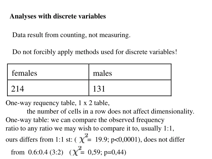
1. Analyses with discrete variables Data result from counting, not measuring. Do not forcibly apply methods used for discrete variables! females males One-way requency table, 1 x 2 table, the number of cells in a row does not affect dimensionality. One-way table: we can compare the observed frequency ratio to any ratio we may wish to compare it to, usually 1:1, ours differs from 1:1 st: ( = 19.9; p<0,0001), does not differ from 0.6:0.4 (3:2) ( = 0,59; p=0,44)

2. A two-way frequency table: we can study associations between two variables: males females black white let’s start from thinking what does it mean that there is no association.

3. Calculate marginal distributions: there is no association when cell frequencies are producs of row and cellfrequencies

4. The same with absolute numbers: These are frequencies for the case when there is no association between the variables.

5. Chi-squared-test in a two-way table looks for the difference from such a table in which there is no association, - tests for a different thing compared to a one-way table.

7. A two-way frequency table: test for an associaton between values of discrete variables There is a statistically significant association between these variables, ( = 85,0; p<0,0001). The strength of the relationship is characterised by odds ratio: (59/103)/(155/28) = 0.103: the “risk” of a black animal to be female is lower.

8. No matter which way to look at it because: (a/b)/(c/d) = (a/c)/(b/d) = ad/cb if there is no association, odds ratio equals 1, one figure is sufficient to describe only in the case of a 2x2 table. Naturally, it is not like that that there should be equal numbers in all cells: 200 100 50 25

9. Assumption of chi-squared test: the expected frequency of any cell should not be below 1, and there should not be more than 20% of cells in which expected frequency is less than 5.

10. An analogous G-test is less sensitive to violation of assumptions, Fisher’s test is not sensitive at all, but Fisher’s test is designed for a very special case, the case when marginal distributions are known in advance: female white female black male black male white • only in a 2x2 table.

11. Athree-way frequency table – rectangular box (cuboid); : 34 37 43 39

12. A three-way frequency table chi-square – is there an association or not, but we want more! Log-linear analysis and interactions:

13. sex*para: division to parasitised andnon-parasitised is not independent of sex; division to females and males is not independent of parasitism; sex*para*year: 1) association between para and year is not independent of sex; 2) association between sex and year is not independent of para; 3) association between sex and pära is not independent of year. There is no distinction between independent and dependent variables! Not frequently needed – too complex sex*year may not be of interest at all!

14. Usually we are interested only in the values of one variable, we can focus on it, declaring it dependent variable, all the rest are independent variables! When binary (has two values) - logistic regression! P=exp(bx+k)/(1+exp(bx+k)) log(P/(1-P) = bx+k; logit(P) = bx + k. probability body weight

15. P=exp(bx+k)/(1+exp(bx+k)) interpretation of parameters (y=0.5 is at –k/b):

16. General linearmodels (ANOVA, ANCOVA....) andgeneralized linear model – other distributions, we can do all the same: • include several independent variables; • include interactions ; • nested, repeated, random. but just more recent – not necessarily available; in addition to binary variable, will consider one more – a variable with Poisson distribution.

17. Values obtained by counting: - bugs on plants; when few – discrete; whan many - continuous; more complicated in between. Poisson distribution: let’s throw grains on chessboard, how many in one field; see the image; small mu: special shape; large mu: approaches normal distribution. characteristic: variance equal to mean; if not: underdispersed or overdispersed, biological reasons.