Download
1 / 53
540 likes | 736 Views
Modeling the 3-D Distribution of Winds in Hurricane Boundary Layer. Yuqing Wang International Pacific Research Center (IPRC) & Department of Meteorology School of Ocean and Earth Science and Technology University of Hawaii at Manoa , Honolulu, HI 96822 September 25, 2012. Outline.

E N D
Modeling the 3-D Distribution of Winds in Hurricane Boundary Layer Yuqing Wang International Pacific Research Center (IPRC) & Department of Meteorology School of Ocean and Earth Science and Technology University of Hawaii at Manoa, Honolulu, HI 96822 September 25, 2012
Outline • Large variability of hurricane boundary layer winds • Surface roughness and orographic effects • An overview of hurricane boundary layer models • A new 3-D hurricane boundary layer model • Proposed development project
Outline • Large variability of hurricane boundary layer winds • Surface roughness and orographic effects • An overview of hurricane boundary layer models • A new 3-D hurricane boundary layer model • Proposed development project
Hurricane Georges (1998) Tangential wind variability near the eyewall in Georges. Kepert (2006a)
Hurricane Georges (1998) Radial wind variability near the eyewall in Georges. Kepert (2006a)
Analyses of the storm-relative Vtrepresentative levels as shown. The contour interval is 5 m/s with heavy labeled contours at multiples of 20 m/s
Analyses of the storm-relative Vrrepresentative levels as shown. The contour interval is 5 m/s with heavy labeled contours at multiples of 20 m/s.
Wind reduction factors. (a) The ratio of the 100-m earth-relative wind speed to that at 1.5 km. (b) The ratio of the 100-m earth-relative wind speed to that at 3 km. Contour interval is 0.05, with multiples of 0.2 heavy and labeled. The white circle shows the approximate RMW and the arrow, the storm motion.
Hurricane Mitch (1998) Tangential wind variability near the eyewall in Mitch. Kepert (2006b)
Hurricane Mitch (1998) Tangential wind variability near the eyewall in Mitch. Kepert (2006b)
Analysis of wind reduction factor, from (a) 1 km to 100 m and (b) 2.5 km to 100 m. Objective analyses of the storm-relative (left) Vt(right) Vrfor levels as shown, based on dropsondedata. Contour interval is 5 m/s, with multiples of 20 m/s shown heavy. Darker shading corresponds to stronger azimuthal wind and stronger inflow, respectively. (Kepert 2006b)
The horizontal analysis of the storm-relative (top) Vtand (bottom) Vr in Hurricane Danielle at heights of 40, 400, and 2000 m. The contour interval is 2 m/s with the heavy labeled contour at multiples of (top) 10 and (bottom) 4 m/s.. The white circles indicate the approximate RMW; the black arrows show the storm motion.
Schematic depicting hurricane boundary layer rolls observed during four hurricane landfalls. Streamline arrows indicate transverse flow, with high (low) momentum air being transported downward (upward). Shaded arrows and bold contours indicate the positive and negative residual velocities.
RADARSAT-1 image of Typhoon Fengshen(2002)showing evidence of fine-scale roll circulations across much of the image. The center of the typhoon is just to the southwest of the image at 28.3N, 140.7E. The image pixel resolution is 150 m.
Variability of hurricane boundary layer winds • Winds in hurricane boundary layer are subject to large variability in both horizontal and vertical directions. • The variability mainly stems from the boundary layer rolls which is triggered primarily by shear instability in the lower part of the boundary layer. • Both horizontal shear and vertical shear are critical to the instability and thus the development of rolls. • The shear is largely determined by the storm structure at the top of the boundary layer, surface roughness and other forcings.
Outline • Large variability of hurricane boundary layer winds • Surface roughness and orographic effects • An overview of hurricane boundary layer models • A new 3-D hurricane boundary layer model • Proposed development project
Topographic speed-up effect, a factor proportional to the height and shape of the terrain, which is as large as 2, used in wind engineering
Downslope wind associated with the small mountains in Tropical Cyclone Larry’s circulation. Ramsay and Leslie (2008)
The 3-hourly accumulated precipitation in gray shading with a 25-mm contour interval for the CTRL TC (left) at (a) 2300, (b) 0200, and (c) 0500 UTC, and for the NOTOPOG TC (right) at (d) 0009, (e) 0309, and (f) 0609 UTC, 2006, for Tropical Cyclone Larry. Terrain elevation is shown by dark gray contours with a contour interval of 100 m. Ramsay and Leslie (2008)
Blocking and channeling effects of small mountains in stable conditions.
An example of orographic effect of Maui on rainfall distribution. An example of blocking and channel effect of Maui orography on surface wind distribution.
6 6 Another type of channel effect of a mountain with hurricane winds parallel to the mountain slope.
Another type of orographic channel effect due to the hurricane winds enter the narrow channel between two mountains.
Close-up of southeast coast of Bermuda showing identified structures with damaged roofs in relation to the underlying topography induced by Hurricane Fabian (2003). Miller et al. (2012)
Surface roughness & orographic effects • Surface roughness determines the surface drag, the inflow angle in the boundary layer, the vertical shear in the surface layer, and thus affect rolls and gustiness. • Orography significantly affects the 3-D distribution of winds under a hurricane. This includes the elevated speed-up effect, slope winds, channel effect between terrain and a hurricane, and channel flow between terrains. • Orography also affects the surface rainfall distribution under hurricane conditions, and thus flooding and landslide etc.
Outline • Large variability of hurricane boundary layer winds • Surface roughness and orographic effects • An overview of hurricane boundary layer models • A new 3-D hurricane boundary layer model • Proposed development project
An overview of hurricane boundary layer models • One-dimensional model #Using a reduction factor to estimate the surface wind based on flight level wind. #Using the logarithm profile based on surface roughness length (may include the orographic speed-up effect). • 2-dimensional slab boundary layer model #including nonlinear effects but assuming a constant boundary layer depth to model the boundary layer mean winds • 3-dimensional boundary layer model Only the model I coded about 12 years ago. It is hydrostatic and it can only be applied to flat surface in its design, and no nesting. • High-resolution full physics model Too expensive to run, in particular the vertical resolution could not be as high as required for applications due to its huge computation of complex model physics.
One type of 1-D model Modeled maximum 1-minute mean wind speeds at a height of 10 m accounting for change of surface roughness effects only under effect of Hurricane Fabian (2003). (Miller et al. 2012)
One type of 1-D model Modeled maximum 1-minute mean wind speeds at a height of 10 m accounting for change of surface roughness and topographic effects combined under effect of Hurricane Fabian (2003). (Miller et al. 2012)
3-Dimensional boundary layer model In hydrostatic, impressible approximations, the equations can be written as
2-D slab-boundary layer model Depth averaged equations (slab boundary layer model equations) can be written as
Difference in the simulated asymmetric distribution of radial and tangential winds for a westward-moving (5 m/s) storm. (Kepert 2010)
The simulated storm-relative (a) 10-m Vt, (b) 10-m Vr, and (c) 1-km w for the model calculation of Mitch. The coastline is shown by the line at y 80 km. Heavy and light contour intervals are (a) 10 and 5 m/s, (b) 5 and 2.5 m/s, and (c) 1 and 0.5 m/s.
(a) Radius–height section of the azimuthal mean storm-relative Vtdivided by the gradient wind, from the model simulation of the boundary layer flow in Hurricanes Georges (left) Mitch (right). Contour interval is 0.05, the contour of 1.0 is heavy, and the vertical white line shows the position of the RMW. (b) Storm-relative gradient wind speed (heavy, m/s) and absolute angular momentum (light, 105 m2s-1).
Modeled storm-relative (top) Vtand (bottom) Vrat 40, 400, and 2000 m in Hurricane Danielle.
High-resolution full-physics model Downslope wind associated with the small mountains in Tropical Cyclone Larry’s circulation simulated in a full physics model with 1 km finest resolution in 46 vertical levels. Ramsay and Leslie (2008)
Parameterized maximum surface wind gusts (gray shading with contour interval of 10 m/s) for the CTRL simulation at time (a) 2300 (landfall) and (b) 0100 UTC. The maximum surface wind gusts for the NOTOPOG simulation at time (c) 0009 (landfall) and (d) 0209 UTC.
Outline • Large variability of hurricane boundary layer winds • Surface roughness and orographic effects • An overview of hurricane boundary layer models • A new 3-D hurricane boundary layer model • Proposed development project
A new 3-D hurricane boundary layer model (Wang 2007) Some New Features compared to Kepert & Wang (2001) • Full-compressible, nonhydrostatic equations • Multiply, two-way interactive, moving nesting • Terrain-following coordinate • Prognostic TKE and TKE dissipation rate • Include the diurnal variation of surface temperature • Better simulate gravity wave breaking & orographic effect due to the use of nonhydrostatic equations • Easy to achieve high resolution in an interested area due to the multiply-nested meshes
Schematic structure of the flow in a mature hurricane in a steady state where gradient wind balance is seen.
Diurnal variation of the planetary boundary layer following Stull (1988)
Perturbation equations from a static atmosphere in a terrain-following vertical coordinate
Nested configuration of the new model 54km 241X141 145X145 18km 6km 145X145 2km 217X217
Deriving the boundary layer model from the full-physics model • Specify the top boundary conditions as a moving steady pressure field representing a hurricane vortex; • Re-derive the coefficients for the triangle metric equations for the semi-implicit vertical motion and pressure perturbation equations based on zero-gradient at the top of the model; • Build in switch on/off between the full physics and moist related process run and dry boundary layer run.