Understanding Imaging Geometry for the Pinhole Camera Model

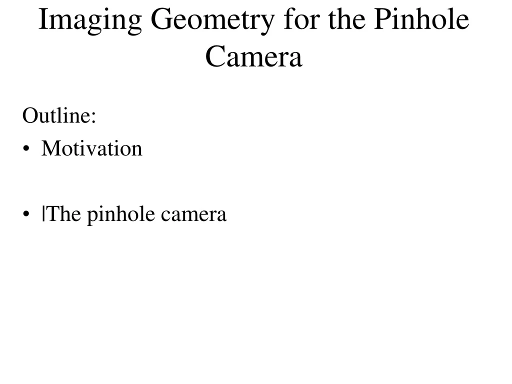
1. Imaging Geometry for the Pinhole Camera Outline: • Motivation • |The pinhole camera

2. Example 1: Self-Localisation View 3 View 1 View 2

3. Example 2: Build a Panorama(register many images into a common frame) M. Brown and D. G. Lowe. Recognising Panoramas. ICCV 2003

4. Example 3: 3D Reconstruction: Detect Correspondences and triangulate

5. Example 4: Camera motion tracking ⇒ image stabilizationbackground part of the image registered original stabilized original stabilized

6. Example 5: Medical imaging – non-rigid image registration for change detection from the atlas before registration after test slice deform. field

7. Example 6: Recognition and Localisation of Objects • Object Models: • What objects are in the image? • Where are they?

8. Example 7: Inspection and visual measurement(in the registered view angles and lengths can be checked)

9. Imaging Geometry: Pinhole Camera ModelThis part of the talk follows A. Zisserman’s EPSRC9 tutorial • Image formation by common cameras is well modeled by a perspective projection: • If expressed as a linear mapping between homogeneous coordinates: 9

10. Imaging Geometry: Internal camera parameters Moving from image plane (x,y) to (u,v) pixel coordinates: C is the camera calibration matrix. • (u0, v0) is the principal point, the intersection of the optical axis and the image plane • au=f ku, av = f kv define scaling in x and y directions

11. Imaging Geometry: From World to Camera Coordinates The Euclidean transformation (rigid motion of the camera) is described by Xc = R Xw + T. Chaining all the transformations: This defines a 3x4 projection matrix P from Euclidean 3-space to an image:

12. Imaging Geometry: Plane projective transformations Choose the world coordinates so that the plane of the points has zero Z coordinate. The 3x4 projection matrix P reduces to:

13. Image Geometry: Computing Plane Projective Transform1 • The plane projective transform is called a homography • Four point-to-point correspondences define a homography • From the model of pinhole camera, we know the form (» denotes similarity up to scale): or, equivalently:

14. Image Geometry: Computing Plane Projective Transform 2 • Multiplying out: • Each point correspondence defines two constraints: • Two approaches can be used to address the scale ambiguity. We will use the simpler one that sets h33=1. This is OK unless points at infinity are involved

15. Image Geometry: Computing Plane Projective Transform 3 • The constrains from four points can be expressed as a linear (in unknowns hij) into an 8x8 matrix:

16. Removing Perspective Distortion • Have coordinates of four points on the object plane • Solve for H in x’=Hx from the and corresponding image coordinates. • Then x=H-1 x’ • (E.g.) inspect the part, checking distances or angle

17. Taxonomy of planar projective transforms II • Notes: • Properties of the more general transforms are inherited by transformations lower in the table • R = [rij] is a rotation matrix, i.e. R R>=1, also

18. Taxonomy of planar projective transforms I • In many circumstances, we know from the imaging set-up, that the image-to-image transformation is simpler than homography or can be well approximated by a transformation with a lower number of degrees of freedom. • Three types of transforms are commonly encountered: • Euclidean (shifted and rotated, e.g. two flatbed scans of the same image ) • Similarity (shift, rotation, isotropic scaling, e.g. two photos from the same spot with different zoom) • Affine transformation

19. Image Geometry: Computing Affine Transform • An affine transform is defined as: • Each point-to-point correspondence provides to constraints, 3 correspondences are needed to uniquely define the transformation. • Solving the problem requires inversion of a single 3x3 matrix:

20. END