Download
1 / 24
250 likes | 471 Views
Combustion associated noise in central heating equipment. FLAME FRONT DYNAMICS. Department of Mechanical Engineering, Combustion Technology. Luiza Bondar Jan ten Thije Boonkkamp Bob Matheij. Viktor Kornilov Koen Schreel Philip de Goey. 1. 2. 3. 4. Outline. Combustion noise

E N D
Combustion associated noise in centralheating equipment FLAME FRONT DYNAMICS Department of Mechanical Engineering, Combustion Technology Luiza Bondar Jan ten Thije Boonkkamp Bob Matheij Viktor Kornilov Koen Schreel Philip de Goey 1 2 3 4
Outline • Combustion noise • Analytical model • Extension of the model • Results and conclusions • Numerical techniques • Boundary conditions • Conclusions and future plans
Combustion noise “Compact, ultra low NOx, efficient, quiet and minimal maintenance”
Combustion noise Goal of the project • understand combustion noise • develop a model that predicts combustion noise
combustion room Bunsen flames gas flow Combustion noise
Combustion noise http://www.em2c.ecp.fr Laboratoire Energétique Moléculaire et Macroscopique, Combustion, E.M2.C acoustic perturbation flame t t acoustic perturbation acoustic perturbation
z r Combustion noise (flame model) flame surfaceG(r, z, t)=G0 z(r,t) the G-equation G<G0 G>G0 v u
z z(r,ts) r Analytical model • Poiseuille flow, i.e., • constant laminar burning velocity SL z(r,0) v u physical domain
Analytical solution technique • the nonlinear G-equation was solved analytically using the method of characteristics • the method of characteristics transforms the G equation in a system of 5 ODEs that depend on an auxiliary variable σ • the solution of the system gives the expressions in term of elliptic integrals for z(r;σ) and t(r;σ)
Analytical model We need σ(r, t) to find z(r, t) physical domain
Analytical model (Results) • the G-equation only cannot account for the flame stabilisation • a stabilisation process based on the physics of the model was derived to stabilise the flame • the flame stabilises in finite time • the nondimensional stabilisation time is ≈1 independently of the value of • the time needed for a flame to stabilise is directly proportional with and inversely proportional with R • the flame reaches a stationary position that is equal with the steady solution of the G-equation (subject to BC z(δ)=0)
Extension of the model • variation of the flame surface area • variation of the burning velocity due to oscillation of the flame front curvature and flow strain rate • interaction of the flame with the burner rim
Extension of the model curvature strain rate SL SL SL SL stream lines
Extension of the model parameters of the flame G-equation hyperbolic term parabolic term
Extension of the model (Numerical Techniques) Level set method (initialization t=0)
Extension of the model (Numerical techniques) use numerical schemes that deal with steep gradients ENO schemes (Essentially Non Oscillatory) • avoid the production of numerical oscillations near the steep gradients • have high accuracy in smooth regions • computationally cheap in WENO (Weighted ENO) form • boundary conditions are difficult to implement
xi-3 xi-2 xi-1 xi xi+1 xi+2 Extension of the model (Numerical techniques) 2 Example 0 1 WENO convex combination with adaptive weights of the approximations of on the stencils the “smoother” the approximation of the larger the weight
“discontinuous” big values Extension of the model (Boundary conditions) -3 -2 -1 0 1 2 ? ? ?
Extension of the model (Boundary conditions) G(x, y) is the distance from (x, y) to the interface
Extension of the model (Examples) external flow velocity expansion in the normal direction
Extension of the model (Examples) shrinking with breaking (normal direction) collapsing due to the mean curvature
Extension of the model (Examples) oscillation of a flame front due to velocity perturbations
Extension of the model (Conclusions) • a high order accuracy numerical scheme was implemented and tested to capture the dynamics of the flame front (C++ and Numlab ) • a good method to implement the boundary conditions was found • current research involves applying the method to the Bunsen flame problem
Extension of the model (Conclusions) • treat the flame with the “open curve” approach • input from Lamfla • analyze and compare the results with the experiments