Download

1 / 69
690 likes | 956 Views
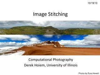
10/19/10. Image Stitching. Computational Photography Derek Hoiem, University of Illinois. Photos by Russ Hewett. Last Class: Keypoint Matching. 1. Find a set of distinctive key- points . 2. Define a region around each keypoint . A 1. B 3.

E N D
10/19/10 Image Stitching Computational Photography Derek Hoiem, University of Illinois Photos by Russ Hewett
Last Class: Keypoint Matching 1. Find a set of distinctive key- points 2. Define a region around each keypoint A1 B3 3. Extract and normalize the region content A2 A3 B2 B1 4. Compute a local descriptor from the normalized region 5. Match local descriptors K. Grauman, B. Leibe
Last Class: Summary • Keypoint detection: repeatable and distinctive • Corners, blobs • Harris, DoG • Descriptors: robust and selective • SIFT: spatial histograms of gradient orientation
Today: Image Stitching • Combine two or more overlapping images to make one larger image Add example Slide credit: Vaibhav Vaish
Panoramic Imaging • Higher resolution photographs, stitched from multiple images • Capture scenes that cannot be captured in one frame • Cheaply and easily achieve effects that used to cost a lot of money • Like HDR and Focus Stacking, use computational methods to go beyond • the physical limitations of the camera
Pike’s Peak Highway, CO Photo: Russell J. Hewett Nikon D70s, Tokina 12-24mm @ 16mm, f/22, 1/40s
Pike’s Peak Highway, CO Photo: Russell J. Hewett (See Photo On Web)
Software • Panorama Factory (not free) • Hugin (free) • (But you are going to write your own, right?)
360 Degrees, Tripod Leveled Photo: Russell J. Hewett Nikon D70, Tokina 12-24mm @ 12mm, f/8, 1/125s
Howth, Ireland Photo: Russell J. Hewett (See Photo On Web)
Capturing Panoramic Images • Tripod vs Handheld • Help from modern cameras • Leveling tripod • Gigapan • Or wing it • Image Sequence • Requires a reasonable amount of overlap (at least 15-30%) • Enough to overcome lens distortion • Exposure • Consistent exposure between frames • Gives smooth transitions • Manual exposure • Makes consistent exposure of dynamic scenes easier • But scenes don’t have constant intensity everywhere • Caution • Distortion in lens (Pin Cushion, Barrel, and Fisheye) • Polarizing filters • Sharpness in image edge / overlap region
Handheld Camera Photo: Russell J. Hewett Nikon D70s, Nikon 18-70mm @ 70mm, f/6.3, 1/200s
Handheld Camera Photo: Russell J. Hewett
Les Diablerets, Switzerland Photo: Russell J. Hewett (See Photo On Web)
Macro Photo: Russell J. Hewett & Bowen Lee Nikon D70s, Tamron 90mm Micro @ 90mm, f/10, 15s
Side of Laptop Photo: Russell J. Hewett & Bowen Lee
Considerations For Stitching • Variable intensity across the total scene • Variable intensity and contrast between frames • Lens distortion • Pin Cushion, Barrel, and Fisheye • Profile your lens at the chosen focal length (read from EXIF) • Or get a profile from LensFun • Dynamics/Motion in the scene • Causes ghosting • Once images are aligned, simply choose from one or the other • Misalignment • Also causes ghosting • Pick better control points • Visually pleasing result • Super wide panoramas are not always ‘pleasant’ to look at • Crop to golden ratio, 10:3, or something else visually pleasing
Ghosting and Variable Intensity Photo: Russell J. Hewett Nikon D70s, Tokina 12-24mm @ 12mm, f/8, 1/400s
Ghosting From Motion Photo: Bowen Lee Nikon e4100 P&S
Motion Between Frames Photo: Russell J. Hewett Nikon D70, Nikon 70-210mm @ 135mm, f/11, 1/320s
Gibson City, IL Photo: Russell J. Hewett (See Photo On Web)
Mount Blanca, CO Photo: Russell J. Hewett Nikon D70s, Tokina 12-24mm @ 12mm, f/22, 1/50s
Mount Blanca, CO Photo: Russell J. Hewett (See Photo On Web)
Problem basics • Do on board
Basic problem • x = K [R t] X • x’ = K’ [R’ t’] X’ • t=t’=0 • x‘=Hxwhere H = K’ R’ R-1 K-1 • Typically only R and f will change (4 parameters), but, in general, H has 8 parameters . X x x' f f'
Views from rotating camera Camera Center
Image Stitching Algorithm Overview • Detect keypoints • Match keypoints • Estimate homography with four matched keypoints (using RANSAC) • Project onto a surface and blend
Image Stitching Algorithm Overview • Detect keypoints (e.g., SIFT) • Match keypoints (most similar features, compared to 2nd most similar)
Computing homography Assume we have four matched points: How do we compute homographyH? Direct Linear Transformation (DLT)
Computing homography Direct Linear Transform • Apply SVD: UDVT= A • h = Vsmallest (column of V corr. to smallest singular value) Matlab [U, S, V] = svd(A); h = V(:, end);
Computing homography Assume we have four matched points: How do we compute homographyH? Normalized DLT • Normalize coordinates for each image • Translate for zero mean • Scale so that average distance to origin is sqrt(2) • This makes problem better behaved numerically (see Hartley and Zisserman p. 107-108) • Compute H using DLT in normalized coordinates • Unnormalize:
Computing homography • Assume we have matched points with outliers: How do we compute homographyH? Automatic Homography Estimation with RANSAC
RANSAC: RANdomSAmple Consensus Scenario: We’ve got way more matched points than needed to fit the parameters, but we’re not sure which are correct RANSAC Algorithm • Repeat N times • Randomly select a sample • Select just enough points to recover the parameters • Fit the model with random sample • See how many other points agree • Best estimate is one with most agreement • can use agreeing points to refine estimate
Computing homography • Assume we have matched points with outliers: How do we compute homographyH? Automatic Homography Estimation with RANSAC • Choose number of samples N • Choose 4 random potential matches • Compute H using normalized DLT • Project points from x to x’ for each potentially matching pair: • Count points with projected distance < t • E.g., t = 3 pixels • Repeat steps 2-5 N times • Choose H with most inliers HZ Tutorial ‘99
Automatic Image Stitching • Compute interest points on each image • Find candidate matches • Estimate homographyH using matched points and RANSAC with normalized DLT • Project each image onto the same surface and blend
Choosing a Projection Surface Many to choose: planar, cylindrical, spherical, cubic, etc.
Planar vs. Cylindrical Projection Planar Photos by Russ Hewett
Planar vs. Cylindrical Projection Cylindrical
Planar vs. Cylindrical Projection Cylindrical
Planar Cylindrical
Recognizing Panoramas Brown and Lowe 2003, 2007 Some of following material from Brown and Lowe 2003 talk
Recognizing Panoramas Input: N images • Extract SIFT points, descriptors from all images • Find K-nearest neighbors for each point (K=4) • For each image • Select M candidate matching images by counting matched keypoints (m=6) • Solve homographyHij for each matched image
Recognizing Panoramas Input: N images • Extract SIFT points, descriptors from all images • Find K-nearest neighbors for each point (K=4) • For each image • Select M candidate matching images by counting matched keypoints (m=6) • Solve homographyHij for each matched image • Decide if match is valid (ni > 8 + 0.3 nf ) # keypointsin overlapping area # inliers
RANSAC for Homography Initial Matched Points
RANSAC for Homography Final Matched Points