Download
1 / 68
680 likes | 695 Views
I. Spatial & Temporal Properties (cont.) II. Signal and Noise. BIAC Graduate fMRI Course October 11, 2005. Spatial and Temporal Properties of BOLD fMRI. Why do you need to know?. Spatial resolution Trades off with coverage Influences viability of preprocessing steps

E N D
I. Spatial & Temporal Properties (cont.)II. Signal and Noise BIAC Graduate fMRI Course October 11, 2005
Why do you need to know? • Spatial resolution • Trades off with coverage • Influences viability of preprocessing steps • Influences inferences about distinct ROIs • Temporal resolution • Tradeoffs between number of slices and TR • Needed resolution depends upon design
What spatial resolution do we want? • Hemispheric • Lateralization studies • Selective attention studies • Systems / lobic • Relation to lesion data • Centimeter • Identification of active regions • Millimeter • Topographic mapping (e.g., motor, vision) • Sub-millimeter • Ocular Dominance Columns • Cortical Layers
What determines Spatial Resolution? • Voxel Size • In-plane Resolution • Slice thickness • Spatial noise • Head motion • Artifacts • Spatial blurring • Smoothing (within subject) • Coregistration (within subject) • Normalization (within subject) • Averaging (across subjects) • Functional resolution
K – Space Revisited . . . . . . . . . . . . . . . . . . . . B A . . . . . . . . . . . . . . . . . . . . . . . . . . . . . . . . . . . . . . . . . . . . . . . . . . . . . . . . . . . . . . . . . . . . . . . . . . . . . . . . . . . . . . . . . . . . . . . . . . . . . . . . . FOV: 10cm, Pixel Size: 2 cm FOV: 10 cm, Pixel Size: 1 cm To increase spatial resolution we need to sample at higher spatial frequencies.
Costs of Increased Spatial Resolution • Acquisition Time • In-plane • Higher resolution takes more time to fill K-space (resolution ~ size of K-space) • #Slices/second • Sample rates for 64*64 images • Early Duke fMRI: 2-4 sl/s • GE EPI: 12 sl/s • Duke Spiral: 14 sl/s • Duke Inverse Spiral: 21+ sl/s • Reduced signal per voxel • What is our dependent measure?
How large are functional voxels? = ~.08cm3 5.0mm 3.75mm 3.75mm Within a typical brain (~1300cm3), there may be about 20,000 functional voxels.
How large are anatomical voxels? = ~.004cm3 5.0mm .9375mm .9375mm Within a typical brain (~1300cm3), there may be about 300,000+ anatomical voxels.
T2* Blurring • Signal decays over time needed for collection of an image • For standard resolution images, this is not a critical issue • However, for high-resolution (in-plane) images, the time to acquire an image may be a significant fraction of T2* • Under these conditions, multi-shot imaging may be necessary.
Partial Volume Effects • A single voxel may contain multiple tissue components • Many “gray matter” voxels will contain other tissue types • Large vessels are often present • The signal recorded from a voxel is a combination of all components
Early examples of ocular dominance Red = Left eye Blue = Right eye Pixel size 0.5mm2 Menon et al., 1997
Reliability of Ocular Dominance Measurements • Cheng et al., 2001 • Same subject participated in two sessions • Raw data at left • Boundaries of dominance columns match well across sessions
Example: Ocular Dominance Goodyear & Menon, 2001
4sec 10sec Goodyear & Menon, 2001
Example: Visual System 100ms 500ms 1500 ms
What temporal resolution do we want? • 10,000-30,000ms: Arousal or emotional state • 1000-10,000ms: Decisions, recall from memory • 500-1000ms: Response time • 250ms: Reaction time • 10-100ms: • Difference between response times • Initial visual processing • 10ms: Neuronal activity in one area
Basic Sampling Theory • Nyquist Sampling Theorem • To be able to identify changes at frequency X, one must sample the data at (least) 2X. • For example, if your task causes brain changes at 1 Hz (every second), you must take two images per second.
Aliasing • Mismapping of high frequencies (above the Nyquist limit) to lower frequencies • Results from insufficient sampling • Potential problem for long TRs and/or fast stimulus changes • Also problem when physiological variability is present
Costs of Increased Temporal Resolution • Reduced signal amplitude • Shorter flip angles must be used (to allow reaching of steady state), reducing signal • Fewer slices acquired • Usually, throughput expressed as slices per unit time
Frequency Analyses t < -1.96 t < +1.96 McCarthy et al., 1996
Phase Analyses • Design • Left/right alternating flashes • 6.4s for each • Task frequency: • 1 / 12.8 = 0.078 McCarthy et al., 1996
Why do we want to measure differences in timing within a brain region? • Determine relative ordering of activity • Make inferences about connectivity • Anatomical • Functional • Relate activity timing to other measures • Stimulus presentation • Reaction time • Relative amplitude
Timing Differences across Regions Presented left hemifield before right hemifield (0-1000ms delays) fMRI vs RT (LH) Plot of LH signal as function of RH signal fMRI vs. Stimulus Menon et al., 1998
Activation maps Relative onset time differences Menon et al., 1998
Timing of mental events measured by fMRI • Miezin et al., 2000 • Subjects pressed button with one hand at onset of 1.5s stimulus • Then, pressed another button at offset of stimulus
V1 FFG Huettel et al., 2001
Secondary Visual Cortex (FFG) Primary Visual Cortex (V1) Subject 1 5.5s 4.0s Subject 2 Huettel et al., 2001
Width of fMRI response increases with duration of mental activity From Menon and Kim, 1999; after Richter et al, 1997
Independence of Timing and Amplitude Adapted from Miezin et al. (2000)
Linear Systems • Scaling • The ratio of inputs determines the ratio of outputs • Example: if Input1 is twice as large as Input2, Output1 will be twice as large as Output2 • Superposition • The response to a sum of inputs is equivalent to the sum of the response to individual inputs • Example: Output1+2+3 = Output1+Output2+Output3
Linear and Non-linear Systems A B C D
Possible Sources of Nonlinearity • Stimulus time course neural activity • Activity not uniform across stimulus (for any stimulus) • Neural activity Vascular changes • Different activity durations may lead to different blood flow or oxygen extraction • Minimum bolus size? • Minimum activity necessary to trigger? • Vascular changes BOLD measurement • Saturation of BOLD response necessitates nonlinearity • Vascular measures combining to generate BOLD have different time courses From Buxton, 2001
Effects of Stimulus Duration • Short stimulus durations evoke BOLD responses • Amplitude of BOLD response often depends on duration • Stimuli < 100ms evoke measurable BOLD responses • Form of response changes with duration • Latency to peak increases with increasing duration • Onset of rise does not change with duration • Rate of rise increases with duration • Key issue: deconfounding duration of stimulus with duration of neuronal activity
Boynton et al., 1996 Varied contrast of checkerboard bars as well as their interval (B) and duration (C).
Differences in Nonlinearity across Brain Regions Birn, et al, 2001