Download
1 / 57
570 likes | 680 Views
Next Topic, Brute Force. Let’s go measure a lot of redshifts, assume z tells us the distance, and see what we can see. => The “z machine of Huchra and Geller. Degrees across the sky. Velocity. Great wall. The Coma cluster. void. Latest and Greatest. “Blow up” of Great Wall.

E N D
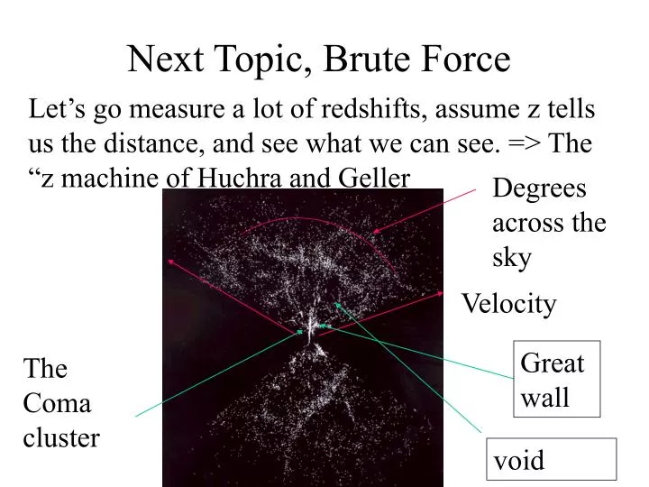
Next Topic, Brute Force Let’s go measure a lot of redshifts, assume z tells us the distance, and see what we can see. => The “z machine of Huchra and Geller Degrees across the sky Velocity Great wall The Coma cluster void
“Blow up” of Great Wall http://www.angelfire.com/id/jsredshift/grtwall.htm
The Next Great Leap Forward: Sloan Goal to really tie down how the light is distributed. A million redshifts @$80/redshift! [Make no small plans No results from this yet, but lots of other neat stuff which we won’t talk about.]
Generate is a “Power Spectrum” Do with galaxies just by “blindly assuming” redshift gives distance and all galaxies “created equal,” i.e no correction for galaxy mass. http://astro.estec.esa.nl/Planck/report/redbook/146.htm We generate the “power spectrum” by measuring the apparent (based on redshift and trigonometry), the distance to the next galaxy, the next and the next. We build up the information on the probability of finding the next galaxy and the next galaxy at a certain distance.
Concept: xxxxxxxxx Number of Objects xxxxxx => xxxxx xx Separation distance
CMB over laid Galaxies “shape parameter” is needed to go from fluctuations in “brick wall” to galaxies See that G = 0.25 is not consistent with Wb =0.05, Wm =1, h = 0.5; more reason for us to assume L > 0 to have a flat universe. G = Wmhexp[-Wb(1 + sqrt(2h)/Wm)]n; JP, page481
As of a few years ago; the CMB derived values are the boxes The galaxy “power” data are the vertical lines CDM model doesn’t fit all! Fits CBM but not galaxies <= larger scales this way Figure 1.13: The boxes in the left hand panel show constraints on the power spectrum P(k) of the matter distribution in an universe implied by observations of the microwave background anisotropies (adapted from White et al. 1994). The points show the power spectrum of the galaxy distribution determined from various galaxy surveys (see Efstathiou 1996). The right hand panel illustrates the accuracy with which PLANCK will be able to determine the power spectrum. The solid curve shows the matter power spectrum expected in an inflationary cold dark matter (CDM) universe. The dotted curve shows a theoretical prediction for a `mixed dark matter' (MDM) universe consisting of a mixture of CDM (60%), massive neutrinos (30%) and baryons (10%).
Update: 2001 Real space galaxy power spectrum of PSCz. Data: correlated power spectrum (version of October 2001). Data: decorrelated linear power spectrum. The dashed line is the flat LCDM concordance model power spectrum from Tegmark, Zaldarriaga & Hamilton (2001), nonlinearly evolved according to the prescription of Peacock & Dodds (1996). The model fits well at linear scales, but fails dismally at nonlinear scales. The PSCz power spectrum requires scale-dependent bias: all unbiased Dark Matter models (Eisenstein & Hu 1998, 1999; Ma 2000) are ruled out with high confidence. Real space correlation function of PSCz. Data: correlation function (version of October 2001). The dashed line is a power law (r / 4.27 h-1Mpc)-1.55. Prewhitened power spectrum of PSCz. Data: prewhitened power spectrum. The solid line is the (unprewhitened) power spectrum. The dashed line is the linear LCDM concordance model power spectrum from Tegmark, Zaldarriaga & Hamilton (2001). The prewhitened nonlinear power spectrum appears intriguingly similar to the linear power spectrum, as remarked by Hamilton (2000). It is not clear whether the similarity has some physical cause, or whether is is merely coincidental.
Basic point of the previous slide is that in theory the measurements of the density fluctuations in the CMB and galaxies are tied together and one model needs to fit all. And it is difficult to measure both on an overlapping length scale. Galaxies are easier to measure on the relatively small scales, CMB on large ones. For the CMB, the z = 1000 means that today the CBM scale as been stretched by 1000 => That’s the problem.
Bottom line: Power spectrum of galaxies is difficult to measure and harder to simulate. So far, we have no good answers. Walls,voids, and power spectra of galaxies require theorists to “fine tune” (dare we say “fudge”?) their models, but there seems no way out for now. And getting CMB, Wb , Wt, and galaxies to all fit is difficult.
Using H0 and distance indicators, the classic tests (1) Number of objects versus redshift (2) Luminosity distance versus redshift (3) Angular size versus redshift
Number of objects versus z The name this goes by is “logN logS”, this is because the range is so large we need to use logs for our ; and which reduces to a straight line if plotted as logS and “S” because this was the way radio people labeled the apparent brightness.
LogN LogS For a Euclidean universe the total number see out to a certain limiting sensitivity ( lowest possible value of S) goes as S-(3/2), easy to show for standard candle case. Without the details, S goes as L/4pD2 for a fixed L and the Volume we are observing to goes as D3 => our exponent [solve for D in terms of S and substitute in to the N = density x (4/3) p D3 equation] is then -3/2
This never worked until recently Because of: “Evolution”. The number of objects per unit volume and the intrinsic luminosity changes. This test failed when we used radio sources. (Because radio is relatively cheap and easy we used radio first.) Rich clusters of galaxies are so “simple” we think we can calculate the evolution, however, and we’ve done this. (cf. The first third of the course) To do the test correctly you have to be sure that you are always comparing the objects with the same intrinsic brightness (implies they are the same physically = size and mass) => be careful
Apparent brightness versus z This has apparently been worked out, i.e. supernovae! But nothing else because the distant objects are different from nearby ones and we can’t predict (model) how. Some math details For L = 0 it is relatively easy to derive a relationship between dL and Omega and z dL= (4c/H0W02)x[zW0/2 + (W0/2-1)(-1 sqrt(W0z+1)] dL is called the Luminosity Distance and clearly depends of W and z and scales as H0
Apparent brightness versus z The one key point is that 4pdL2 is what we divide the luminosity by to predict a flux,F and then we assume we have a standard candle and we know L and then we compare predicted F with observed F.
Abundances: Why is this important for Cosmology? Because He/H, D/H, and Li/H are all predicted by BB nucleosynthesis The values of these ratios that we measure can then be used to infer Wb which we can use to infer there must be WIMPs
Key Concepts Need to be sure the region we observe is close to “primodial” = the initial stuff left over form the BB. The reason we can’t use measurement of abundaces here on Earth.. There have been too many changes. No need for you to know them all. Need to be sure you are counting all the atoms which can be “hidden”: for example , ionized, atomic, and molecular H all give different “finger prints”
Key Concepts, cont. Atoms can absorb (absorption lines) and re-radiate light (emission lines). Only certain kinetic energy values are allowed (this is Quantum Mechanics; take it as given here) for the electrons circling the nucleus. Cool Atom model
We use both absorption and emission line studies Emission lines are generally harder to come by because the gas has to supply the light were as we can look for a bright “light bulb” that shines through cooler (means there are atoms with electrons in orbits that are low enough to absorb the light and make “lines”
Real live examples: Stars Hotter interior Cooler atmosphere
Absorption lines are the darker regions MK Types White O5V B1V A1V F3V G2V K0V M0V
Key to inferring the element type is the spacing of the lines. Key to inferring the amount is the darkness (and width) of the lines. Key to interpretation: must assume atoms haven’t been created or destroyed.
Helium Two places to look: star atmospheres and the interstellar medium. He is nice because it is chemically inert, so we don’t have to worry about it’s being bound up. Helium is also nice because it has a very stable nucleus and is not likely to be destroyed. It might be created, however since H is burned into He in stars. => look for the lowest values we can find
How low can you go? Part I Concept is that Oxygen was made after the BB, so the presence of O is a measure of contamination Make a measure of He/H versus O/H and “extrapolate to “zero” O. And look at stellar atmospheres
A delicate measurement SN only go to here
“How low can you go?”, Part II He/H is defined as Y
More on definition of Y There are 2 ways to measure ratio, by mass and by number. When astronomers measure by mass, they call the ratio Y, and for all the elements heavier than He, astronomers call these elements “metals” and call the ratio of metals/H = Z. How do we convert from mass to number for He?
More on definition of Y Y= mass of He/(mass of He + mass of H + mass of metals) ; assume metals are negligible Or Y = mHex NHe/(mHex NHe+mH x NH) Take mHe = 4mH, and mH =1, and substitute in, then do algebra. Find that if Y = 0.25 = 1/4, that NHe/NH = 1/12 or about 8% => 25% by mass is equivalent to 8% by number => Always be sure to ask, by mass or by number
Deuterium What is it? It is chemically just like ordinary H. It is an “isotope” of H which means D has the same number of protons in its nucleus, but a different number of neutrons. In this case, just one neutron for D, and zero for H.
Deuterium D/H has proven very difficult to measure. Why? Three reasons at least: (1) D is rare (D/H about 0.01% by number, because not much was left over from BB (2) D is easily destroyed in stellar atmospheres so we can’t use stars or our very own ISM. (3) The spectral “finger print” is only very slightly shifted with respect to H.
Deuterium The finger print is almost the same because the only difference is one neutron in the nucleus, and this has no charge. Remember D and H both have one electron orbiting the nucleus. The only effect is with mass, not charge. The electron’s orbital distance from the nucleus is slightly different (about 1 part in 1000 smaller)
Deuterium How to see this without too much math? Concept is “center of mass”, and the more massive the nucleus, the closer the center of mass will be to it. This means for the same separation, since both orbit the center of mass, the electron will go faster for the heavier nucleus case since the nucleus travels a smaller circle to follow around. This means it needs to get closer to the nucleus so the electrical force can hold it to balance the centrifugal force (higher v = higher centrifugal force for a given radius). Means stronger electric pull, means bluer (more energetic line)
Round ‘n Round Electron must always be exactly opposite the nucleus along the Center of mass line, by definition . The H nucleus (proton) is over 1000 times more massive than the electron, so even doubling the mass of the nucleus isn’t going to move the nucleus in much closer to the center of mass. Therefore the effect is SMALL. Center of mass Proton + neutron nucleus motion Proton motion Electron motion Electron motion H exaggerated D, exaggerated
Consequence of small effect: Need a very good prism and a very strong “light bulb” behind the absorbing material. And star atmospheres can’t work because D can be destroyed there.Also, Interstellar medium D comes from stars => also depressed below primoridal values. Furthermore, the main effect is only slight shift, not a real change in the pattern. => Deuterium lines look like “blue shifted” H, and we have to hope we have made the right identification.
Deuterium, OK where to look? Find distant ( highs z = > 1) bright light bulbs = QSOs, that through clouds of gas in between galaxies that we think are “primodial” and therefore have not had D reduced by star processing First try looked good, but they seem to have been wrong!
data Models in blue
models D/H = 0 D/H = 3.4 x10⁻⁵ D/H = 25 x10-5 Better result? data Location of D line center if no H present
Li Lithium is so rare we can only look for it in stars, but it is easily destroyed so the results are uncertain
Predictions and results (Ratio of baryons/photons) (Ratio of baryons/photons)
Agreement? There results barely agree within errors (uncertainties), but we still think Big Bang Nucleuosynthesis is OK
Star cluster dating Assume all the stars in a cluster formed at the same time Assume we know how stars evolve, know how long they spend as stable stars such as our sun does.
Star cluster dating Assume all the stars in a cluster formed at the same time Assume we know how stars evolve, so we know how long they spend as stable stars such as our sun does.
Star Cluster Dating The keys is that L is proportional to M and also proportional to the surface T, so that we know that kind of star we are looking at by either measuring it’s color (or if dust messes us up, the lines for the gases that will be different depending on the T; more later)
Star Cluster Dating See page 128 of book Stars here live the shortest time Log(L) The lower this point, the older the cluster “Main sequence” Log(T)
Analogy Assuming no re-seeding but that it started with marigolds ( an annual) and roses (a perennial) and we find one garden with marigolds we know it is less than 1 year old, and conversely, one without is at least 1 year old.