Download
1 / 22
350 likes | 666 Views
Classical Statistical Mechanics: Paramagnetism in the Canonical Ensemble. Paramagnetism. Paramagnetism occurs in substances where the individual atoms, ions or molecules possess a permanent magnetic dipole moment . The permanent magnetic moment is due to the contributions from:

E N D
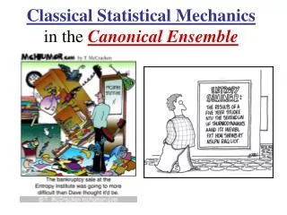
Classical Statistical Mechanics: Paramagnetism in the Canonical Ensemble
Paramagnetism Paramagnetism occurs in substances where the individual atoms, ions or molecules possess a permanent magnetic dipole moment. The permanent magnetic moment is due to the contributions from: 1. The Spin(intrinsic moments) of the electrons.
Paramagnetism Paramagnetism occurs in substances where the individual atoms, ions or molecules possess a permanent magnetic dipole moment. The permanent magnetic moment is due to the contributions from: 1. The Spin(intrinsic moments) of the electrons. 2. The Orbital motion of the electrons.
Paramagnetism Paramagnetism occurs in substances where the individual atoms, ions or molecules possess a permanent magnetic dipole moment. The permanent magnetic moment is due to the contributions from: 1. The Spin(intrinsic moments) of the electrons. 2. The Orbital motion of the electrons. 3. The Spinmagnetic moment of the nucleus.
Some Paramagnetic Materials • Some Metals. • Atoms, & moleculeswith an odd number • of electrons, such as free Na atoms, • gaseous Nitric oxide (NO) etc. • Atoms or ionswith a partly filled inner • shell: Transition elements, rare earth & • actinide elements. Mn2+, Gd3+, U4+ etc. • A few compounds withan even number • of electrons including molecular oxygen.
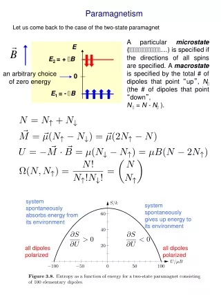
Classical Theory of Paramagnetism • Consider a material with N • magnetic dipolesper unit • volume, each with moment . • In the presence of a magnetic • field B, the potential energy • of a magnetic dipole is:
This shows that the • dipoles tend to line up • with B. B = 0 M = 0 B ≠ 0 M ≠ 0 • The effect of temperature is to randomize • the directions of the dipoles. • The effect of these 2 competing processes • is that some magnetization is produced.
Suppose that B is applied along • the z axis, so that is the angle • made by the dipole with the z • axis as shown in the figure. • The Canonical Ensemble Probability of • finding the dipole along the direction is • proportional to the Boltzmann factor f():
The Canonical Ensemble Probability • of finding the dipole in the direction • is proportional to: • The average value of z then is given by: • The integration is carried out over the solid • angle with element d. It thus takes into • account all possible orientations of the dipoles.
To do the integral, substitute • z = cos & d = 2 sin d • which gives: So:
Let cos = x, then sin d = - dx & limits -1 to +1 Then: And:
So, the mean value of z has the form: “Langevin Function” L(a) So: z
The mean value of z is thus: Langevin Function, L(a) z • In most practical situations, a < < 1, so • So, in this limit, the approximate magnetization is N = Number of dipoles per unit volume
The mean value of z : Langevin Function, L(a) z • For small a < < 1 Variation of L(a) with a. • In this limit, the • magnetization is
For small a < < 1 • This is known as the “Curie Law”. The susceptibility • is referred as theLangevinparamagnetic susceptibility. • It can be written in • in a simplified form as: Curie constant
All of this was obtained using the Canonical • Ensemble & treating the magnetic dipoles classically. • Our results are that the magnetization has the form: • l • By contrast, earlier, we used the Canonical Ensemble • & treated the magnetic dipoles quantum • mechanically assuming spin s = ½ . We found that the • magnetization in this case has the form: M = N z with z
The magnetization M & its dependence on the • dimensionless energy ratio • are obviously not the same • for the two cases. However, it is worth noting that the • function M(x)displays similar qualitative behavioras • a function of x in the two cases. a x
The magnetization M & its dependence on the • dimensionless energy ratio • are obviously not the same • for the two cases. However, it is worth noting that the • function M(x)displays similar qualitative behavioras • a function of x in the two cases. • Specifically, in the small x limit, (low B, high T), in • both cases, the magnetization simplifies to M = B • where is called the magnetic susceptibility. a x
The magnetization M & its dependence on the • dimensionless energy ratio • are obviously not the same • for the two cases. However, it is worth noting that the • function M(x)displays similar qualitative behavioras • a function of x in the two cases. • Specifically, in the small x limit, (low B, high T), in • both cases, the magnetization simplifies to M = B • where is called the magnetic susceptibility. • It can be written in the “Curie Law” form a x Further, C has the same form in both models!!
So, both the Classical Statistics model & the • Quantum (spin s = ½)model give the same • magnetizationM & in the small x limit, (low • B, high T). That is, both cases give M = B. • Also, the susceptibility has the Curie “Law” form: a x
So, both the Classical Statistics model & the • Quantum (spin s = ½)model give the same • magnetizationM & in the small x limit, (low • B, high T). That is, both cases give M = B. • Also, the susceptibility has the Curie “Law” form: a x • Further, both models give the same qualitative result for • the magnetizationMin the large x limit, (high B, low T). • That is, both cases give M Constant as x . In • other words, for large enough x, in both models the • magnetizationMsaturates to a constant value called • the Saturation Magnetization.
A side by side comparison of plots of the magnetization • M as a function of x for the two cases just discussed • illustrate the behavior discussed for both small & large x. “Saturation Magnetization” M = B. M = B. Quantum (Spin ½ ) Result Classical Result