Download
1 / 27
400 likes | 954 Views
Simple linear regression and correlation analysis. Regression Correlation Significance testing. 1. Simple linear regression analysis. Simple regression describes relationship between two variables Two variables, generally Y = f(X) Y = dependent variable (regressand)

E N D
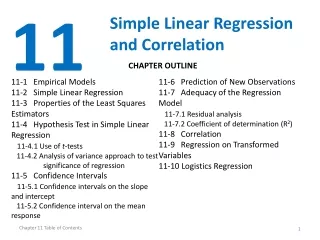
Simple linear regression and correlation analysis Regression Correlation Significance testing
1. Simple linear regression analysis • Simple regression describes relationship between two variables • Two variables, generally Y = f(X) • Y = dependent variable (regressand) • X = independent variable (regressor)
Simple linear regression • f (x) – regression equation • ei – random error, residual deviation • independent random quantity • N (0, σ2)
Simple linear regression – straight line • b0 = constant • b1 = coefficient of regression
Parameter estimates →least squares condition • difference of the actual Y from the estimated Y est. is minimal • hence n is number of observations (yi,xi) • adjustment under partial derivation of function according to parameters b0, b1, derivation of the S sum of squared deviationas are equated to zero:
Two approches to parameter estimates with using of least squares condition (made for straight line equation) • Normal equation system for straight line • Matrix computation approach • y = dependent variable vector • X = independent variable matrix • b = vector of regression coefficient (straight line → b0 and b1) • ε = vector of random values
Simple linear regression • observation yi • smoothed values yi est; yi´ • residual deviation • residual sum of squares • residual variance
Simple lin. reg. → dependence Y on X • Straight line equation • Normal equation system • Parameter estimates – computational formula
Simple lin. reg. → dependence X on Y • Associated straight line equation • Parameters estimates – computational formula
2. Correlation analysis • corr. analysis measures strength of dependence – coeff. of correlation „r“ • │r│is in<0; +1> • │r│is in<0; 0,33> weak dependence • │r│is in<0,34; 0,66> medium strong dependence • │r│is in<0,67; 1> strong to very strong dependence • r2 = coeff. of determination, proportion (%) of variance Y, that is caused by the effect of X
Significance test of parameters b1 (straight line) (two-sided) • test criterion • estimate sb for par. b1 • table value (two-sided) if test criterion>table value→H0 is rejected and H1 is valid; if test alfa>p-value→H0 is rejected
Coefficient of regression estimation • interval estimate for the unknown βi
Significance test of coeff. corr. r (straight line) (two-sided) • test criterion table value (two-sided) if test criterion>table value→H0 is rejected and H1 is valid; if test alfa>p-value→H0 is rejected
Coefficient of correlation estimation • small samples and not normal distribution • Fischer Z – transformation • first r is assigned to Z (by tables) • interval estimate for the unknown σ • last step Z1 a Z2 is assigned to r1 a r2
The summary ANOVA (alternatively) • test criterion • table value
Multicollinearity • relationship between (among) independent variables • among independent variables (X1; X2….XN) is almost perfect linear relationship, high multicollinearity • before model formation is needed to analyze of relationship • linear independent of culumns (variables) is disturbed
Causes of multicollinearity • tendencies of time series, similar tendencies among variables (regression) • including of exogenous variables, delay • using 0;1 coding in our sample
Consequences of multicollinearity • wrong sampling • null hypothesis about zero regression coefficient is not rejected, really is rejected • confidence intervals are wide • regression coeff estimation is very influented by data changing • regression coeff can have wrong sign • regression equation is not suitable for prediction
Testing of multicollinearity • Paired coefficient of correlation • t - test • Farrar-Glauber test • test criterion • table value if test criterion>table value→H0 is rejected
Elimination of multicollinearity • variables excluding • get new sample • once again re-formulate and think out the model (chosen variables) • variables transformation – chosen variables recounting (not total consumption, but consumption per capita… etc.)
Regression diagnostics • Data quality for the chosen model • Suitable model for the chosen dataset • Method conditions
Data quality evaluation • A) outlying observation in „y“ set • Studentized residuals |SR| > 2 → outlying observation → outlying need not to be influential (influential has cardinal influence on regression)
Data quality evaluation • B) outlying observation in „x“ set • Hat Diag leverage hii – diagonal values of hat matrix H H = X . (XT . X)-1 . XT hii > → outlying observation
Data quality evaluation • C) influential observation • Cook D (influential obs. influence the whole equation) Di > 4 → influential obs. • Welsch – Kuh DFFITS distance (influential obs. influence smoothed observation) |DFFITS| > → influential obs.
Method condition • regression parameters <-∞; +∞> • regression model is linear in parameters (not linear – data transformation) • independent of residues • normal distribution of residues N(0;σ2)