Spectral methods for initial value problems and integral equations

1. Spectral methods for initial value problems and integral equations Tang Tao Department of Mathematics, Hong Kong Baptist University International Workshop on Scientific Computing On the Occasion of Prof Cui Jun-zhi’s 70th Birthday

2. Outline of the talk • Motivations (accuracy in time) • Spectral postprocessing (efficiency) • Singular kernels • Delay-differential equations • Extensions • Joint with Cheng Jin, Xu Xiang (Fudan)

3. We begin by considering a simple ordinary differential equation with given initial value: y’(x) = g(y; x), 0 < x T, (1.1) y(0) = y0. (1.2) Can we obtain exponential rate of convergence for(1.1)-(1.2)? For BVPs, the answer is positive and well known. For the IVP (1.1)-(1.2), spectral methods are not attractive since (1.1)-(1.2) is a local problem A global method requires larger storage and computational time (need to solve a linear system for large T or a nonlinear system in case that g in (1.1) is nonlinear). Spectral postprocessing (Tang and X. Xu/Fudan)

4. Purpose: a spectral postprocessing technique which uses lower order methods to provide starting values. A few Gauss-Seidal type iterations for a well designed spectral method. Aim:to recover the exponential rate of convergence with little extra computational resource. Spectral postprocessing

5. Formulas … We introduce the linear coordinate transformation and the transformations Then problem (1.1)-(1.2) becomes Y’(x) = G(Y; s), 1 < s 1; Y(1) = y0. Let be the Chebyshev-Gauss-Labbato points: We project G to the polynomial space PN: where Fj is the j-th Lagrange interpolation polynomial associated with the Chebyshev-Gauss-Labbato points.

6. Formulas … Since Fj  PN, it can be expanded by the Chebyshev basis functions: Assume it is satisfied in the collocation points , i.e., which gives we finally obtain the following numerical scheme (1.3) where It is noticed that

7. Let be the Legendre-Gauss-Labatto points, we obtain the following numerical scheme (1.4) where Legendre collocation (Lobatto III)

8. Consider a simple example y’ = y + cos(x+1)ex+1, x  (1,1], y(1)=1. The exact solution of the is y=(1+sin(x+1))exp(x+1). First use explicit Euler method to solve the problem (with a fixed mesh size h=0.1). Then we use the spectral postprocessing formulas to update the solutions using the Gauss-Seidal type iterations. Example 1

9. Example 1: errors vs Ns for spectral postprocessing method (1.4), with (a): Euler, (b): RK2, and (c): RK4 solutions as the initial data. (a) (b) (c)

10. Spectral postprocessing for Hamiltonian systems As an application, we apply the spectral postprocessing technique for the Hamiltonian system: (1.5) with the initial valuep(t0) = p0, q(t0) = q0, Feng Kang, Difference schemes for Hamiltonian formalism an symplectic geometry, J. Comput. Math., 4 1986, pp. 279-289. • 4th-order explicit Runge-Kutta • 4th-order explicit symplectic method

11. Spectral postprocessing for Hamiltonian systems Integrating (1.5) leads to a system of integral equation Assume (1.6) holds at the Legendre or Chebyshev collocation points: where tkj = (tk + 1) + j, 0  j  N. We can discretize the integral terms in (1.7) using Gauss quadrature together with the Lagrange interpolation:

12. Consider the Hamiltonian problem (1.5) with This system has an exact solution (p, q) = (sint, cost). We take T=1000 in our computations. Table 1(a) presents the maximum error in t[0,1000] using both the RK4 method and the symplectic method. Table 2(b) shows the performance of the postprocessing with initial data in [tk, t2+2] generated by using RK4 t=0.1). To reach the same accuracy of about 1010, the symplectic scheme without postprocessing requires about 5 times more CPU time. Example 2

13. Example 2. (a): the maximum errors obtained by RK4 and the symplectic method; (b): spectral postprocessing results using the RK4 (t = 0.1) as the initial data in each sub-interval [tk, tk+2]; (c): same as (b), except that RK4 is replaced by the symplectic method. Here N denotes the number of spectral collocation points used.

14. (a) Example 2: errors vs Ns and iterative steps with (a): RK4 results and (b): symplectic results as the initial data. (b)

15. Spectral postprocessing for Volterra integral equations Legendre spectral method is proposed and analyzed for Volterra type integral equations: where the kernel k and the source term g are given. Let be the zeros of Legendre polynomials of degree Ns+1, i.e., LNs+1(x). Then the spectral collocation points are We collocate (1.8) at the above points: Using the linear transform we have

16. Example 4 Consider Eq. (1.8) with Example 4: errors vs Ns and iterative steps.

17. The convergence analysis [Tang, Xu, Cheng/Fudan Univ] Theorem 1Let u be the exact solution of the Volterra equation (1.9) and assume that where uj is given by spectral collocation method and Fj(x) is the j-th Lagrange basis function associated with the Gauss-points If u  Hm(I), then for m  1, provided that N is sufficiently large.

18. Lemma 3.1 Assume that a (N+1)-point Gauss, or Gauss-Radau, or Gauss-Lobatto quadrature formula relative to the Legendre weight is used to integrate the product u, where u  Hm(I), with I:=(1, 1) for some m 1 and  PN. Then there exists a constant C independent of N such that Lemma 3.2 Assume that u  Hm(I) and denote INu its interpolation polynomial associated with the (N+1)-point Gauss, or Gauss-Radau, or Gauss-Lobatto points Then Lemma 3.3 Assume that Fj(x) is the N-th Lagrange interpolation polynomials associated with the Gauss, or Gauss-Radau, or Gauss-Lobatto points. Then The convergence analysis (Proof ingredients)

19. Methods and convergenceanalysis for [Yanping Chenand Tang] • Chebyshev spectral for \alpha=0.5 • Jacobi-spectral for general \alpha

20. Spectral methods for pantograph-type DDEs Ishtiaq Ali (CAS) Hermann Brunner (Newfoundland/HKBU) Tao Tang

21. Consider the delay differential equation: u(x) = a(x)u(qx),0 < x  T, u(0) = y0, where 0 < q < 1 is a given constant … • Using a simple transformation, the above problem becomes y(t) = b(t)y(qt + q1), -1 < t  1, y(-1) = y0.

22. Difficulties in using finite-difference type methods (a). u(qx) – un-matching of the grid points so interpolations are needed – difficult to obtain high order methods (b). Difficult in obtaining stable numerical methods (analysis has been available for q=0.5 only) (c). Difficult when q close to 0 or 1.

24. Theorem: If the function b is sufficiently smooth (which also implies that the solution is smooth), then provided that N is sufficiently large

25. Consider the general pantograph equation with a(t) = sin(t), b(t) = cos(qt), c(t) = -sin(qt), g(t) = cos(t) – sin2(t). The exact solution of the problem isy(t) = sin(t).

26. Figure:L errors for general pantograph equation with neutral term. (a): q = 0.5 and (b): q = 0.99.

27. Spectral methods for fractional diffusion equation(Huang/Xu/Tang) Consider the time fractional diffusion equation of the form subject to the following initial and boundary conditions: u(x,0) = g(x), x , u(0,t) = u(L,t)=0, 0  t  T, where  is the order of the time fractional derivative. is defined as the Caputo fractional derivatives of order  given by

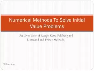
28. Basic equations for Viscoelastic flows where S is an elastic tensor related to the extra-stress tensor of the fluid by is the rate of deformation tensor. The extra-stress tensor is given by an adequate constitutive equation, where the memory function is

29. (a) (b) Predicted streamlines for the flow through a 4:1 planar contraction for Re=1 using the finite volume code of Alves et al. (a) Newtonian; (b) UCM model with We=4.

30. Happy Birthday, Professor Cui!

31. Methods and error analysis for delay equations [H. Brunner/Newfoundland and HKBU and Tang]